How can we effectively characterize the potential for landslide initiation? A landslide inventory shows where landslides have occurred over some period of time. We use the inventory to identify conditions spatially and temporally associated with landslide occurrence. We assume that the landslides in the inventory represent some proportion of the population of all possible landslides and expect that landslides in the future will be associated with similar conditions. We can characterize these associations in terms of density: the number (or area or volume) of observed landslides per unit basin area. We seek to determine landslide density as a function of measurable attributes of the terrain and weather associated with the landslides observed. In most cases, we focus on the terrain because we do not have reliable methods for measuring attributes of the weather associated with landslide occurrence.
Once we have functions describing landslide density in terms of terrain attributes, we can create maps of landslide density based on those attributes. If done well, we should find that most of the observed landslide initiation zones fall within areas of high modeled landslide density, but perhaps not all the initiation zones, because some proportion of the landslides may have occurred in unusual locations. A low modeled density indicates conditions associated with a smaller proportion of the observed landslides. Likewise, we will have zones of high modeled landslide density where there are no observed landslides in our inventory. We expect that the inventory represents only a portion of the entire population of all possible landslides. Areas of high modeled density indicate those zones with conditions similar to the conditions where landslides were observed. We expect that these will be sites of landslide occurrence in the future.
Within the boundaries of the basin or study-area where the landslide inventory was collected, if we integrate the modeled density over that area, the integral will give the number (or area or volume, depending on how the landslide initiation zones where characterized) of landslides within that boundary. The number (area, volume) of inventoried landslides, however, depends on the time period over which the inventory was collected and the landslide-triggering storms that occurred during that period. Density can, therefore, only provide a relative measure of how landslide potential varies over the landscape, showing where conditions associated with a greater or lesser proportion of the landslides in the inventory exist.
To provide an absolute measure of landslide potential, we can translate the density of landslides to the proportion of landslides. Then our maps go from indicating the number (or area or volume) of landslides in the inventory associated with particular terrain attributes to the proportion of landslides in the inventory associated with those attributes. This provides a testable prediction. For any future landslide inventory, we can predict what proportion of observed landslides will occur within any particular portion of a basin or study area. We can then, for example, delineate those locations from which we expect a certain proportion (e.g., 20%) of all landslides will occur, ranked by landslide density.
The goal here is to find functions relating landslide density to terrain attributes. The frequency-ratio method measures density directly. To measure the frequency ratio, construct two cumulative frequency distributions for a single attribute, such as hillslope gradient, one distribution for areas within the initiation zones and another for the entire study area. Then divide the distribution for the initiation zones by the distribution for the entire area. For any increment of hillslope gradient, this ratio gives the proportion of area in the initiation zones; that is, the density as a function of gradient. One can generalize to more than one attribute, but characterizing the frequency distribution of multiple attributes becomes exceeding uncertain and sensitive to any peculiarities in our sample of landslides: we encounter the curse of dimensionality
Frequency ratio is appealing because it uses all the information we can infer about topography from a DEM and is easily interpreted. But we also want to explore relationships with multiple terrain attributes. There are many classification modeling strategies available: logistic regression, random forest, etc., but these require that we extract a sample of points from both the initiation zones and the rest of the study area. The attributes associated with those points are then used to characterize conditions associated with the initiation zones. This characterization is provided as a probability that any location is within an initiation zone. Probability in this case can be interpreted as density. For example, if we randomly sample 100 points from the study area with a modeled probability of 0.7, we expect that 70 will fall inside initiation zones and 30 outside. Density is simply a measure of proportion: 70 points out of 100 gives a density of 0.7. There is uncertainty in what the measured proportion will be, but we can calculate that uncertainty as a function of the probability and the number of points sampled.
Sample points
The issue now is, how to select the sample of points? How many, and how should they be divided between the initiation zones and everywhere else? Given that the initiation zones may cover a fraction of a percent of the study area, it is not immediately obvious how to divvy up the points. An assumption inherent in these classification methods is that the value at any sample point is independent of the value at any other point. Because these methods are ultimately determining proportions (e.g., what proportion of sampled points over a gradient interval of 0.7 to 0.8 fell within initiation zones), if some points are essentially sampling the same location (e.g., the same landslide scar), the calculated proportions will be biased towards values at those locations. How do we ensure that the sampled points provide independent values? Finally, how do our choices about sample selection affect the modeled probabilities?
Independence
How far apart do the sample points need to be to ensure that each provides a measure of terrain attributes independent of the values at any other point? We can look at the degree of autocorrelation for topographic attributes using, e.g., a semivariogram, as we do below, but what does that actually tell us?
Consider a long, planar slope. The elevation changes in a regular fashion along the fall line, but not at all along a contour. The gradient (measured along the fall line) is about the same everywhere on the slope, so the degree of correlation is high. The gradient will decrease at the ridge crest and the base of the slope, so the range on the semivariogram should be about the length of the hillslope. Yet, we may find multiple, separate landslides initiating within lesser distances of each other on the slope. What terrain attributes might be affecting landslide initiation? If we exclude the ridge and base of the slope from calculation of the semivariance, we may find a smaller range (and sill) indicative of minor variations in gradient along the slope. Is this the appropriate separation distance to use?
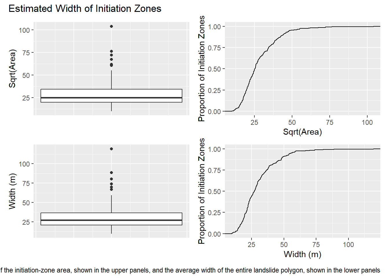
Given our reliance on remotely sensed data, we cannot fully assess the factors that influence landslide initiation and it is probable that some of these factors are not visible with the data we have. These invisible-to-use factors may vary over length scales less than the variations visible in our remotely sensed data, even with high-resolution lidar-derived topography. The size distribution of the landslide scars themselves may offer some insight. Here are boxplots and cumulative frequency distributions of the estimated width of the initiation zones of the 244 landslide polygons used from the Tongass National Forest landslide inventory on Wrangell Island. Width is estimated both as the square root of the initiation-zone surface area and from the average width of the entire landslide polygon.
Code
library(data.table)library(ggplot2)library(patchwork)library(TerrainWorksUtils)library(stringr)# First we need to run LS_poly to build the data files used as inputs for the analyses.dataFolder <-"c:/work/data/wrangell/"DEM <-paste0(dataFolder, "elev_wrangell.flt")polyFile <-paste0(dataFolder, "LS_polys_Wrangell.shp")polyID <-"ID"gradRadius <-7.5diameter <-round(2.*gradRadius,0)gradFile <-paste0(dataFolder, "Grad_", diameter, ".flt")if (file.exists(paste0(gradFile))) { inGrad <- gradFile outGrad <-"nofile"} else { inGrad <-"nofile" outGrad <- gradFile}tanRadius <-15.0diameter <-round(2.*tanRadius,0)tanFile <-paste0(dataFolder, "Tan_", diameter, ".flt")if (file.exists(tanFile)) { inTan <- tanFile outTan <-"nofile"} else { inTan <-"nofile" outTan <- tanFile}profRadius <-15.0diameter <-round(2.*profRadius,0)profFile <-paste0(dataFolder, "Prof_", diameter, ".flt")if (file.exists(profFile)) { inProf <- profFile outProf <-"nofile"} else { inProf <-"nofile" outProf <- profFile}inFoS <-paste0(dataFolder, "FoS_pca6.flt")outNodes <-paste0(dataFolder, "centerNodes")outCSV <-paste0(dataFolder, "outpoly")outInit <-paste0(dataFolder, "init")scratchDir <-"c:/work/scratch/"executableDir <-"c:/work/sandbox/landslideutilities/projects/ls_poly/x64/release"if (!file.exists(paste0(dataFolder, outCSV, "_init.csv"))) { returnCode <- TerrainWorksUtils::LS_poly( DEM, polyFile, polyID, inGrad, inTan, inProf, inFoS, outGrad, gradRadius, outTan, tanRadius, outProf, profRadius, outNodes, outCSV, outInit, scratchDir, executableDir)if (returnCode !=0) { stop("Error in LS_poly, return code: ", returnCode) }}
Code
initStats <-as.data.table(read.csv(paste0(outCSV, "_init.csv")))boxarea <-ggplot(initStats, aes(y=sqrt(Area_m2))) +geom_boxplot() +labs(y ="Sqrt(Area)") +theme(axis.text.x =element_blank(),axis.ticks.x =element_blank())cumarea <-ggplot(initStats, aes(x=sqrt(Area_m2))) +stat_ecdf(geom="step") +labs(x ="Sqrt(Area)",y ="Proportion of Initiation Zones")boxwidth <-ggplot(initStats, aes(y=Width_m)) +geom_boxplot() +labs(y ="Width (m)") +theme(axis.text.x =element_blank(),axis.ticks.x =element_blank())cumwidth <-ggplot(initStats, aes(x=Width_m)) +stat_ecdf(geom="step") +labs(x ="Width (m)",y ="Proportion of Initiation Zones")pwidth <- (boxarea + cumarea) / (boxwidth + cumwidth)pwidth <- pwidth +plot_annotation(title ="Estimated Width of Initiation Zones" ,caption ="Width (m) is estimated as the square root of the initiation-zone area, shown in the upper panels, and the average width of the entire landslide polygon, shown in the lower panels")pwidth
Both measures suggest that about 90% of all initiation zones are 50 m or less in width. Let’s look at some potential predictors. Program samplePoints will read the specified rasters of predictors, find the range of predictor values that fall within the initiation-zone polygons, and create a mask file to exclude areas outside those ranges. This is similar to excluding the ridge top and valley floor with looking at gradient values in the planar-slope example described above. We are examining only those areas with the range of predictor values where landslide initiations were observed. The code chunks below will run samplePoints to create a mask raster and then use the cv_spatial_autocor function from the blockCV package to calculate semivariograms for each predictor raster. The semivariogram will indicate the range of spatial autocorrelation for each predictor.
Code
library(terra, exclude ="resample")# List of predictor rasters, single precision realr1 <-c("Gradient", "c:/work/data/wrangell/grad_15", 0.01, 0.99)r2 <-c("FoS_6", "c:/work/data/wrangell/FoS_pca6", 0., 0.99)r3 <-c("FoS_72", "c:/work/data/wrangell/FoS_pca72", 0., 0.99)r4 <-c("PCA_6", "c:/work/data/wrangell/pca_6", 0., 0.99)r5 <-c("PCA_72", "c:/work/data/wrangell/pca_72", 0., 0.99)r6 <-c("Tan_30", "c:/work/data/wrangell/tan_30", 0.01, 0.99)r7 <-c("Norm_30", "c:/work/data/wrangell/norm_30", 0.01, 0.99)r8 <-c("Mean_30", "c:/work/data/wrangell/mean_30", 0.01, 0.99)R4rasters <-list(r1,r2,r3,r4,r5,r6,r7,r8)for (i in1:length(R4rasters)) { r <- terra::rast(paste0(R4rasters[[i]][2],".flt"))names(r) <- R4rasters[[i]][1]if (i ==1) { rstack <- r } else { rstack <-c(rstack, r) }}
Code
# Run sample points to build a raster masking zones outside the range of predictor values# associated with landslide initiation zones. Edit input variables as neededinRaster <-"c:/work/data/wrangell/init"# initiation zones, raster created by LS_polyareaPerSample <-25000.# within initiation zones, one point every areaPerSample square metersbuffer_in <-10.# buffer around sample points inside initiation zones, in metersbuffer_out <-10.# buffer around sample points outside initiation zonesmargin <-1.# margin around initiation zones to preclude sample points close to the edge, in metersratio <-1.# ratio of sample points outside initiation zones to those withinnbins <-100# number of bins for building histograms# Add landform typei1 <-c("Landform", "c:/work/data/wrangell/newLandform")i2 <-c("Soils", "c:/work/data/wrangell/soils")I4rasters <-list(i1, i2)minPatch <-100000.inPoints <-"c:/work/data/wrangell/inpoints1000"outPoints <-"c:/work/data/wrangell/outpoints"outMask <-"c:/work/data/wrangell/mask"outInit <-"c:/work/data/wrangell/initMod"table <-"c:/work/data/wrangell/table"scratchDir <-"c:/work/scratch"executableDir <-"c:/work/sandbox/landslideutilities/projects/samplepoints/x64/release"returnCode <- TerrainWorksUtils::samplePoints( inRaster, areaPerSample, buffer_in, buffer_out, margin, ratio, nbins, R4rasters, I4rasters, minPatch, inPoints, outPoints, outMask, outInit, table, scratchDir, executableDir)if (returnCode !=0) {stop("Error in samplePoints, return code: ", returnCode)}mask <- terra::rast(paste0(outMask, ".flt"))for (i in1:length(R4rasters)) { rstack[[i]] <- rstack[[i]] * mask}
Code
library(blockCV)library(automap)# Build a semivariogram for each predictor. var <-cv_spatial_autocor(r=rstack, num_sample=100000)
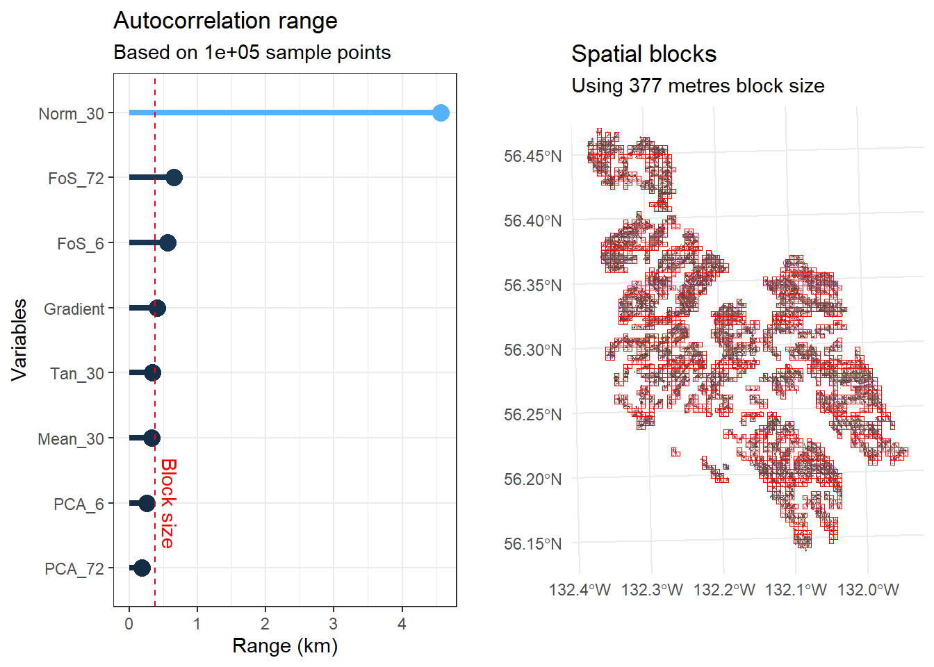
Gradient was calculated over a diameter of 15 meters, thus smoothing variations over length scales less than that. The range of the semivariogram for this measure of gradient is about 300 meters, which is around the midpoint of hillslope lengths included within the mask raster. The two flow accumulation rasters, PCA_5 and PCA_72, indicate the approximate contributing area for each DEM cell for a 5 and 72 hour storm, assuming a saturated hydraulic conductivity of 1 m/sec and ignoring infiltration time. PCA_5 is highly correlated with gradient and has a similar semivariogram range. PCA_72 has flow concentrations within channels and exhibits much larger variability than PCA_5, indicated by its larger range and sill. The factor of safety values (FoS) are derived from the gradient and flow accumulation values. Despite the large differences between PCA_5 and PCA_72, the FoS rasters based on these exhibit similar patterns of variability with nearly equal ranges and sills.
What do these range values imply for our strategy of sampling independent points? They are all several times larger than the typical scale of a landslide initiation zone. Even if we use the ~300-m range found for gradient as the minimum point spacing, that precludes more than one sample point per landslide initiation zone. Ultimately the goal is to have a representative sample that accurately reflects the range and frequency distribution of predictor values across both the observed initiation zones and the masked area spanning the range of values observed within the initiation zones. Independence precludes bias in our representation of those frequency distributions, but bias will still be an issue if we have too few points.
Number
How many randomly placed sample points do we need to obtain an accurate and complete representation of the frequency distribution of predictor values? That depends on how uniform the frequency distributions are. Long-tailed distributions require more points to ensure that rare conditions get samples. We can compare frequency distributions of sample-point sets to those of the predictor rasters. This is straight forward for single predictors, but becomes more complicated when looking at combinations of predictors.
Representative sample, curse of dimensionality.
Single predictors
Let’s start with one sample point per initiation zone and a point spacing of 300m elsewhere. We can generate point samples with program samplePoints.
Code
# Edit input variables as neededinRaster <-"c:/work/data/wrangell/init"# initiation zones, raster created by LS_polyareaPerSample <-282743.# within initiation zones, one point every areaPerSample square metersbuffer_in <-300.# buffer around sample points, in metersbuffer_out <-300.# buffer around sample points outside initiation zonesmargin <-1.# margin around initiation zones to preclude sample points close to the edge, in metersratio <-3.# ratio of sample points outside initiation zones to those withinnbins <-100# number of bins for building histogramsminPatch <-100000.inPoints <-"c:/work/data/wrangell/inpoints_1"outPoints <-"c:/work/data/wrangell/outpoints_1"outMask <-"c:/work/data/wrangell/mask"outInit <-"c:/work/data/wrangell/initMod"table <-"c:/work/data/wrangell/table1"scratchDir <-"c:/work/scratch"executableDir <-"c:/work/sandbox/landslideutilities/projects/samplepoints/x64/release"returnCode <- TerrainWorksUtils::samplePoints( inRaster, areaPerSample, buffer_in, buffer_out, margin, ratio, nbins, R4rasters, I4rasters, minPatch, inPoints, outPoints, outMask, outInit, table, scratchDir, executableDir)
I found building cumulative distributions with R to be rather slow, so program samplePoints also outputs a csv file with a histogram for each of the predictors. We can use these to compare the frequency distributions of the sample points to those of the predictor rasters. The files have five columns:
Lower, the lower bound of the interval
Upper, the upper bound of the interval
Mid, the midpoint of the interval
Number, the number of DEM cells or sample points included in the interval
CumulativeProp, the cumulative proportion of cells or samples
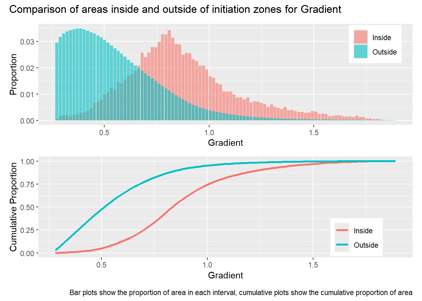
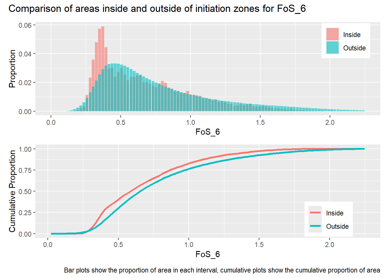
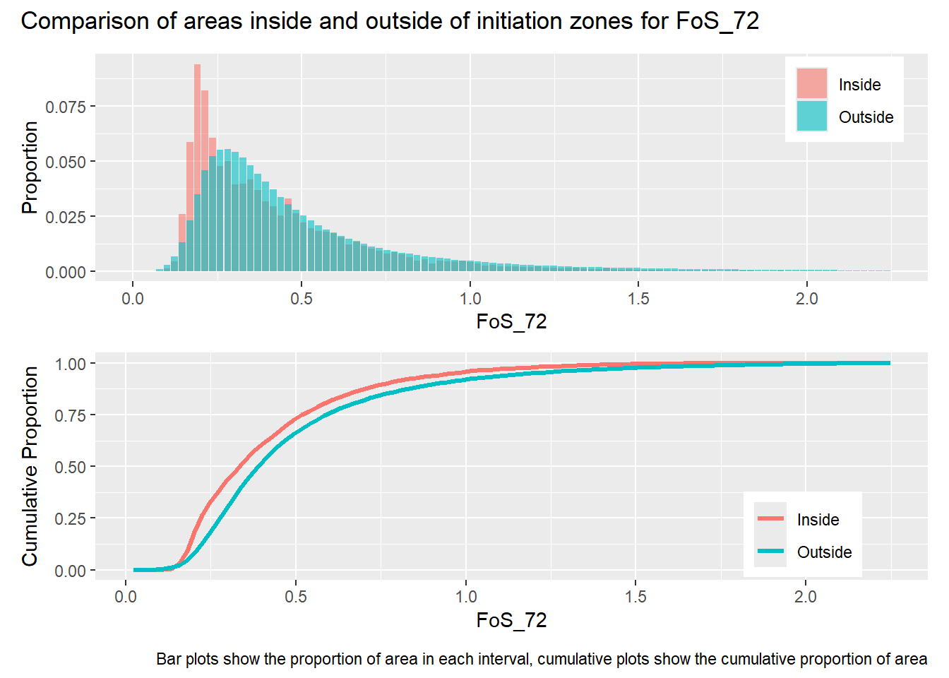
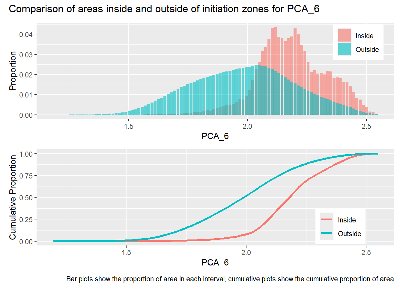
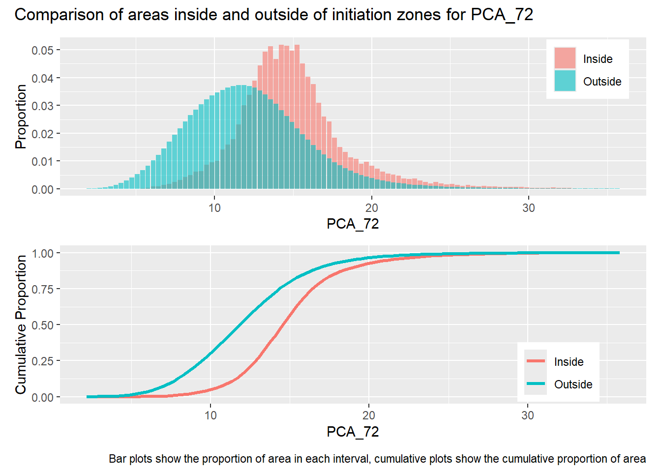
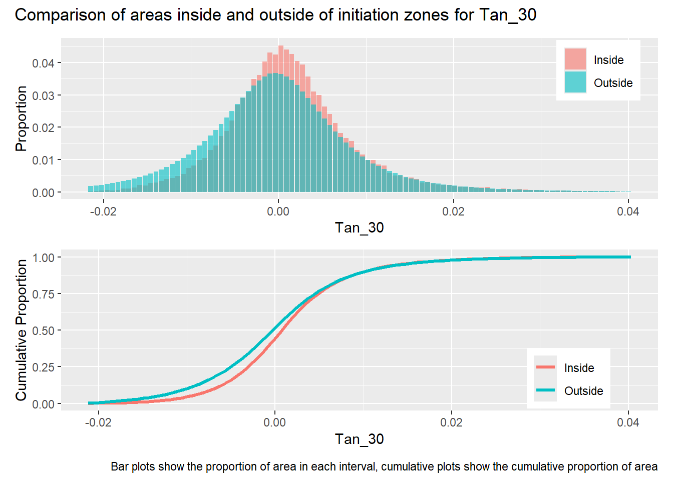
There are two things of interest, examined in the follows plots:
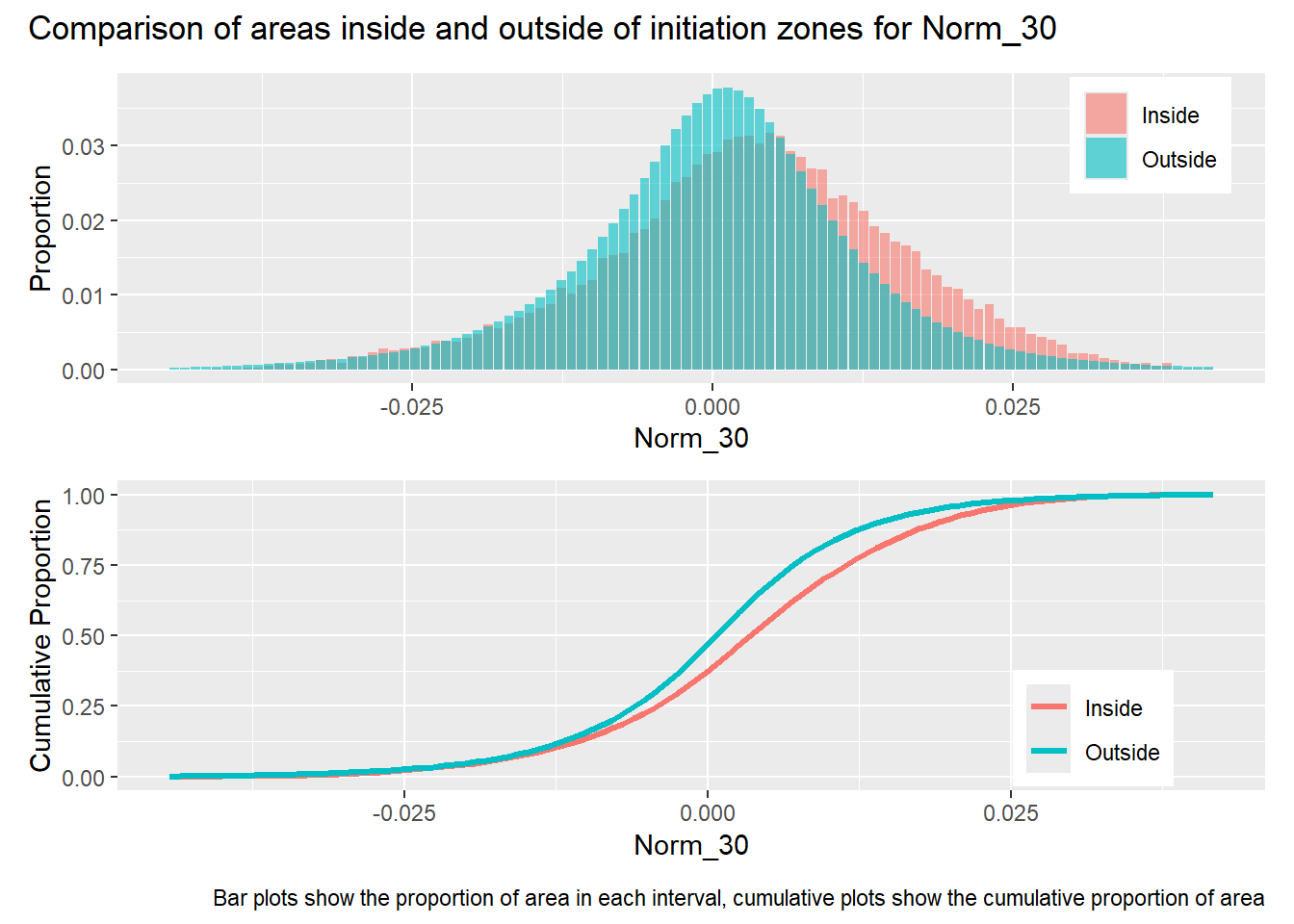
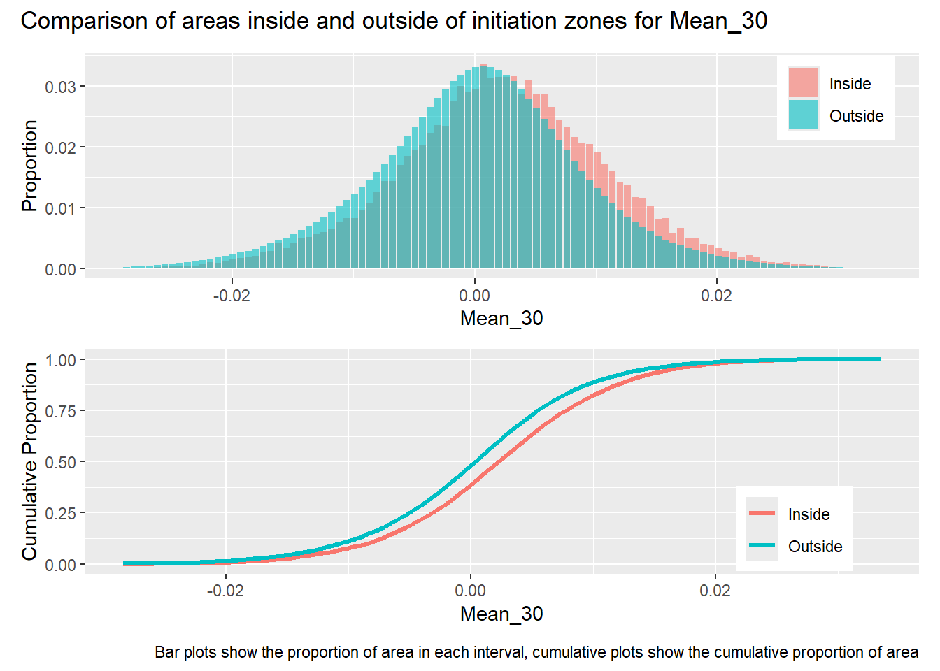
How different, or similar, are the frequency distributions for areas inside and outside of the initiation zones?
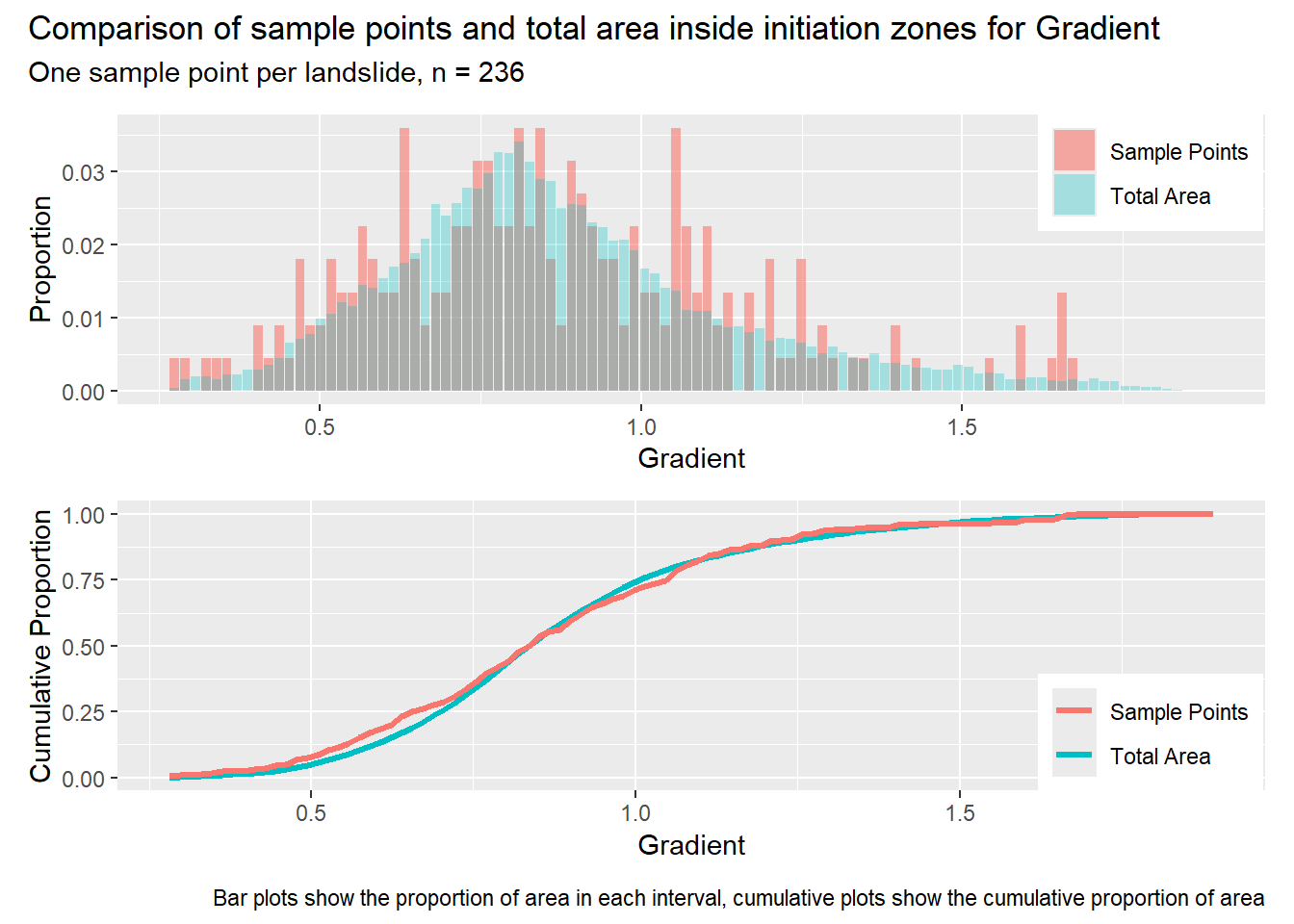
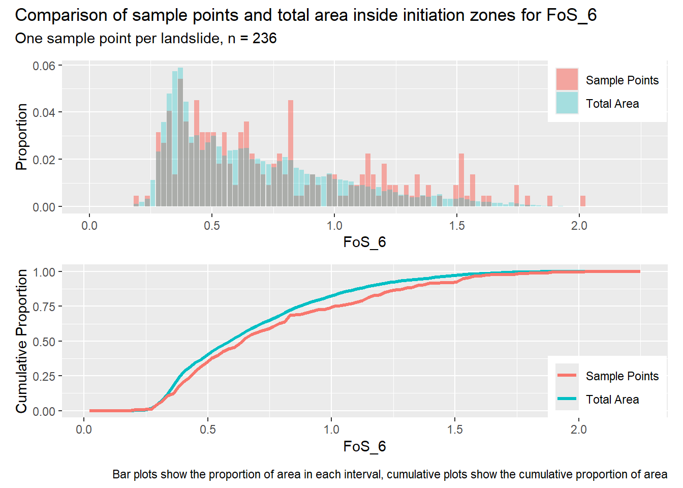
How well do the frequency distributions for the sample points match those of the area sampled?
library(patchwork)#| label: in_vs_outfor (i in1:length(R4rasters)) { thisplot <- pbar[[i]] / pdif[[i]] thisplot <- thisplot +plot_annotation(title =paste0("Comparison of areas inside and outside of initiation zones for ", R4rasters[[i]][[1]]),caption ="Bar plots show the proportion of area in each interval, cumulative plots show the cumulative proportion of area")plot(thisplot)}
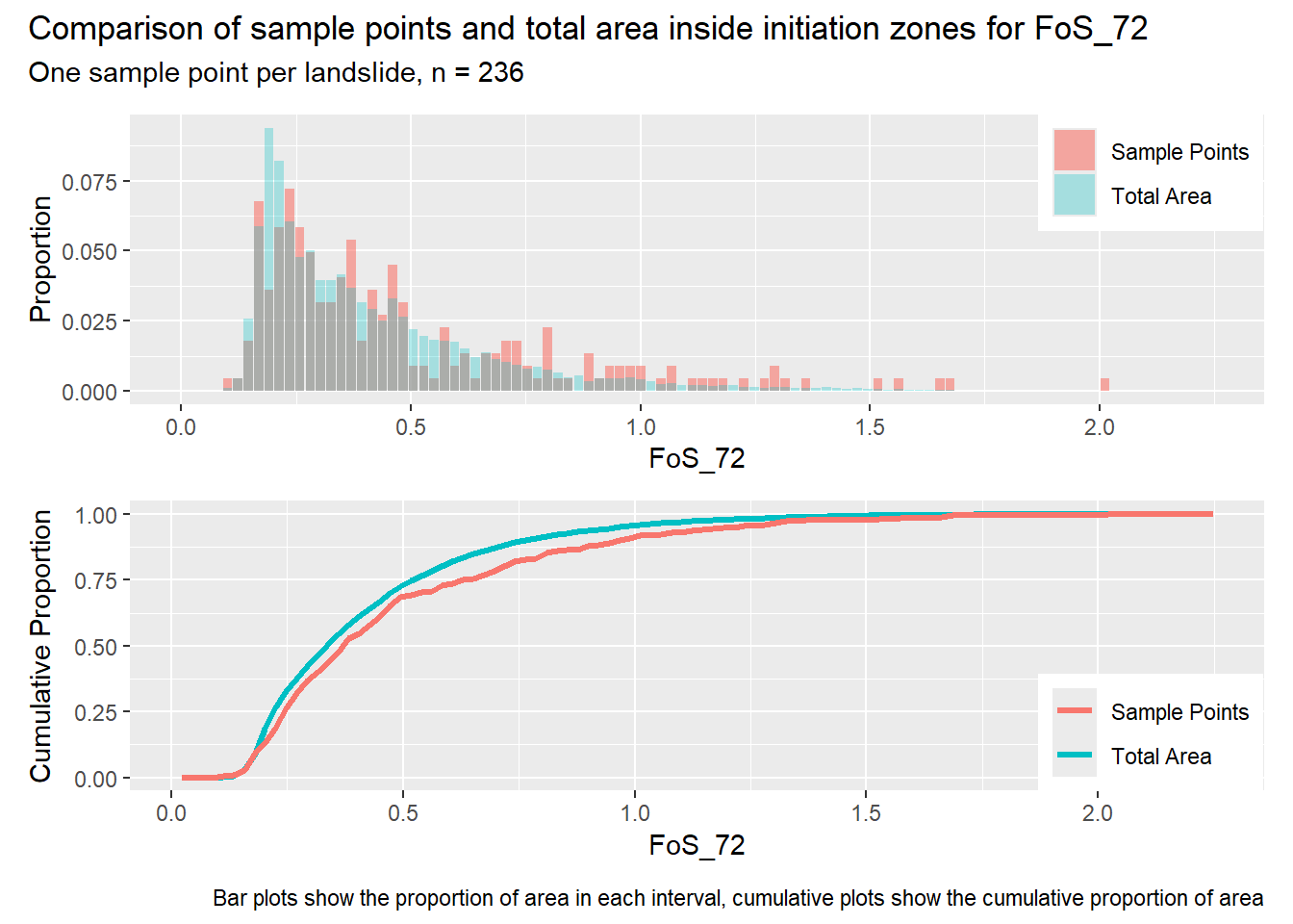
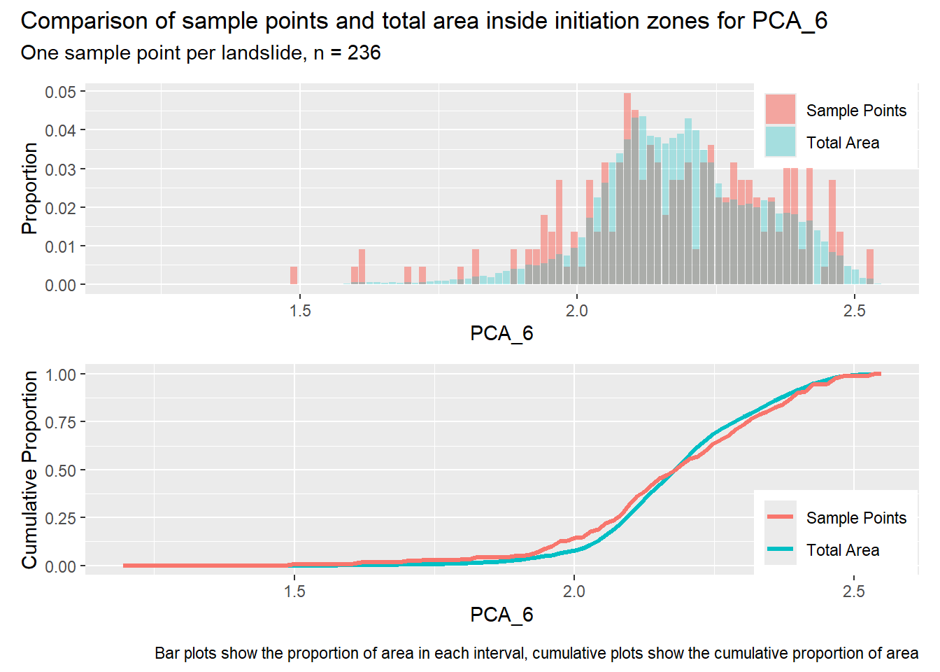
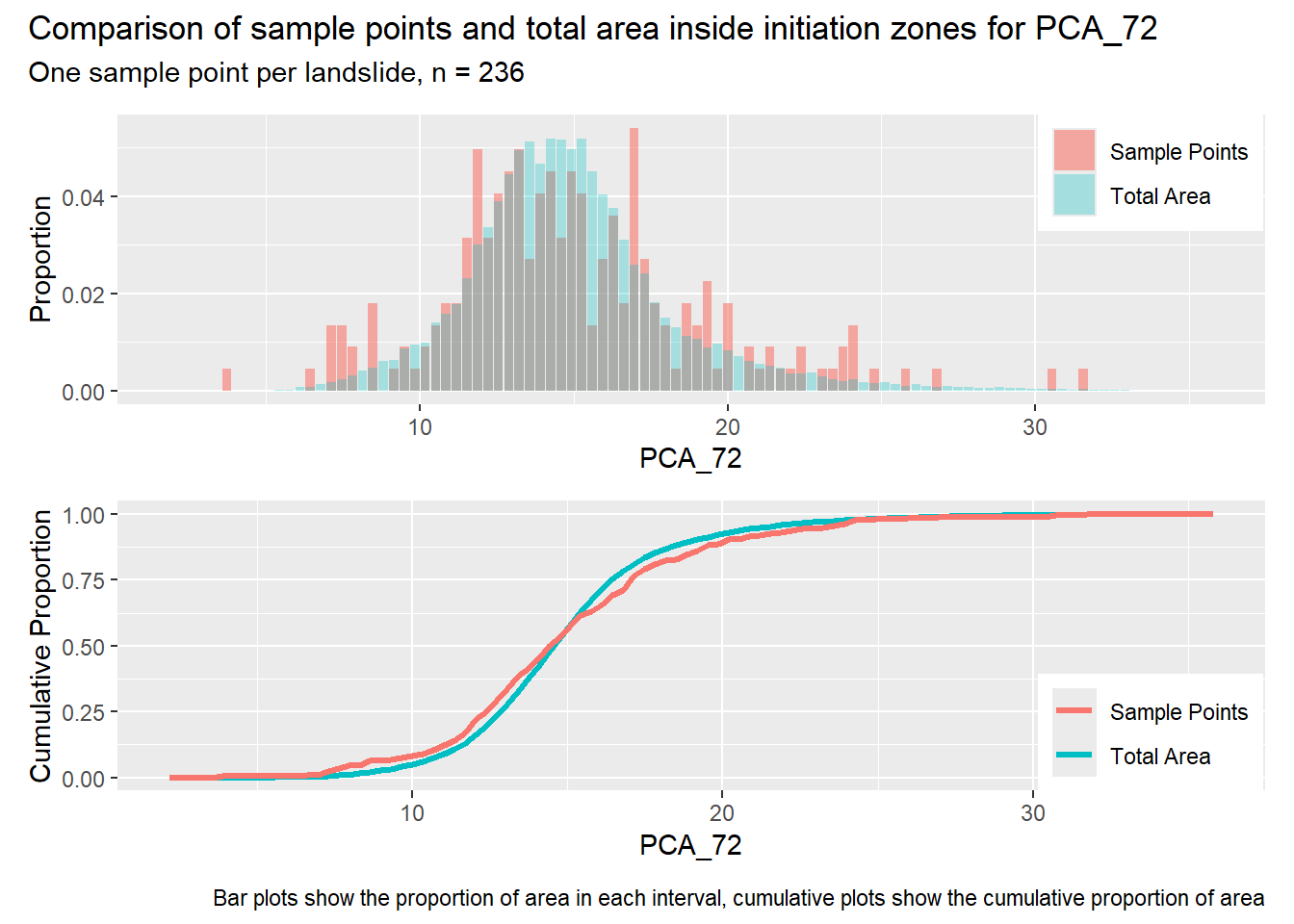
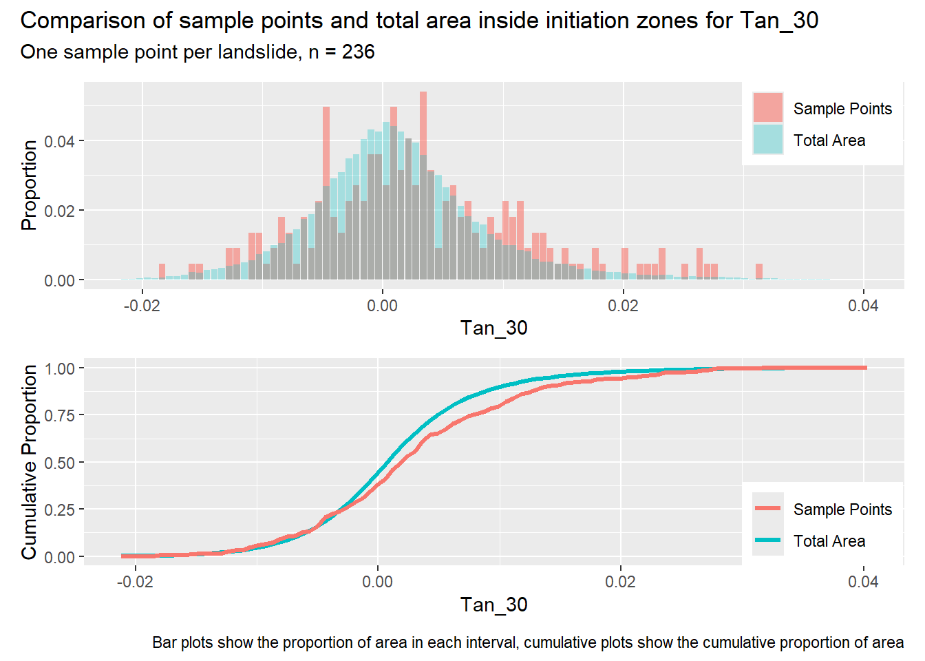
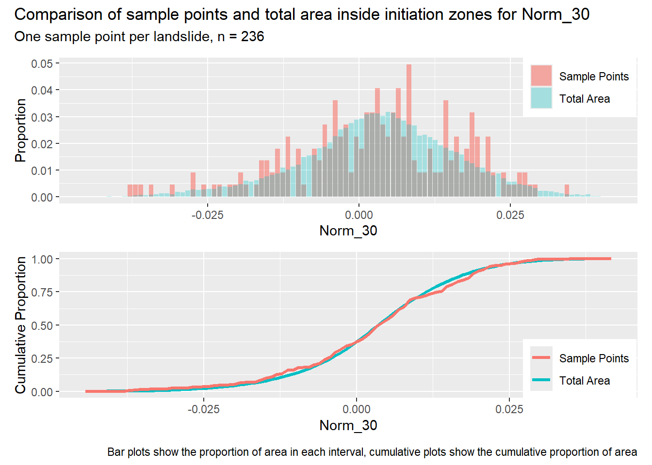
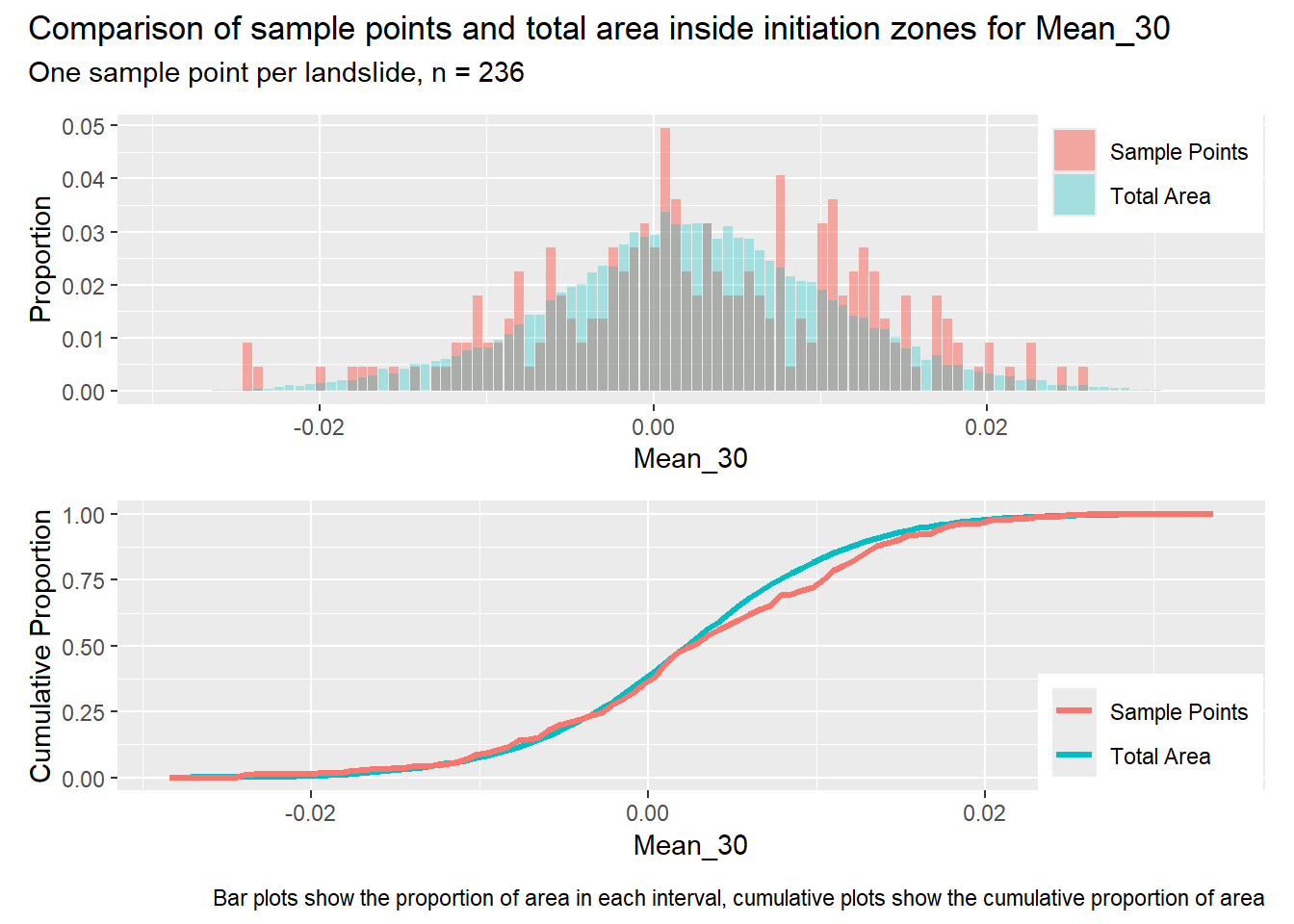
Code
for (i in1:length(R4rasters)) { thisplot <- pbar_in[[i]] / pcum_in[[i]] thisplot <- thisplot +plot_annotation(title =paste0("Comparison of sample points and total area inside initiation zones for ", R4rasters[[i]][[1]]),subtitle ="One sample point per landslide, n = 236",caption ="Bar plots show the proportion of area in each interval, cumulative plots show the cumulative proportion of area")plot(thisplot)}
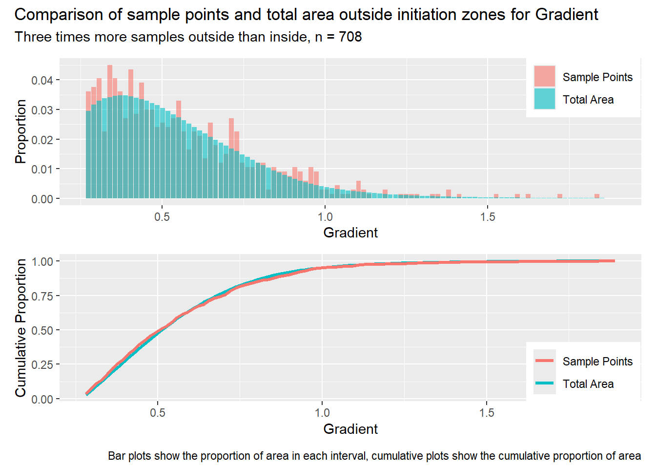
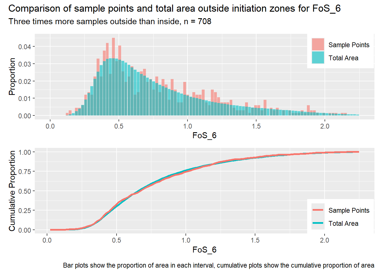
Code
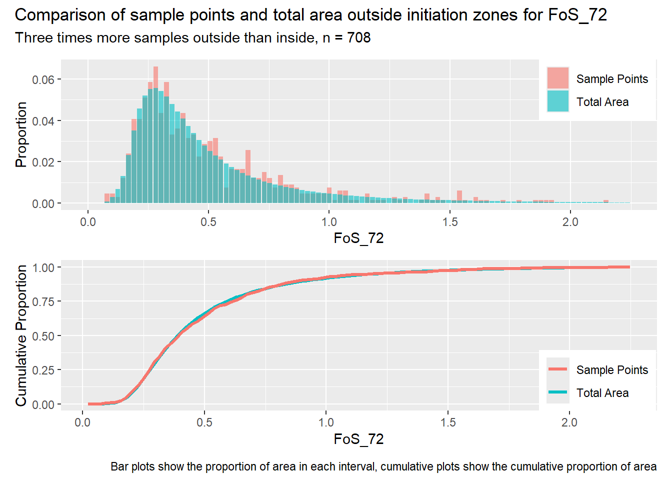
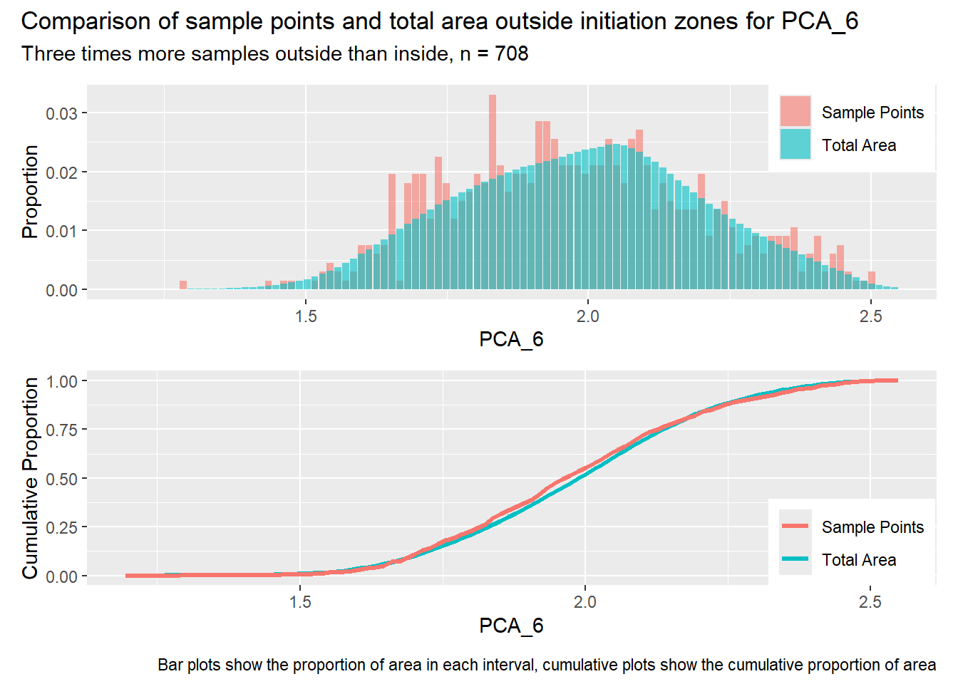
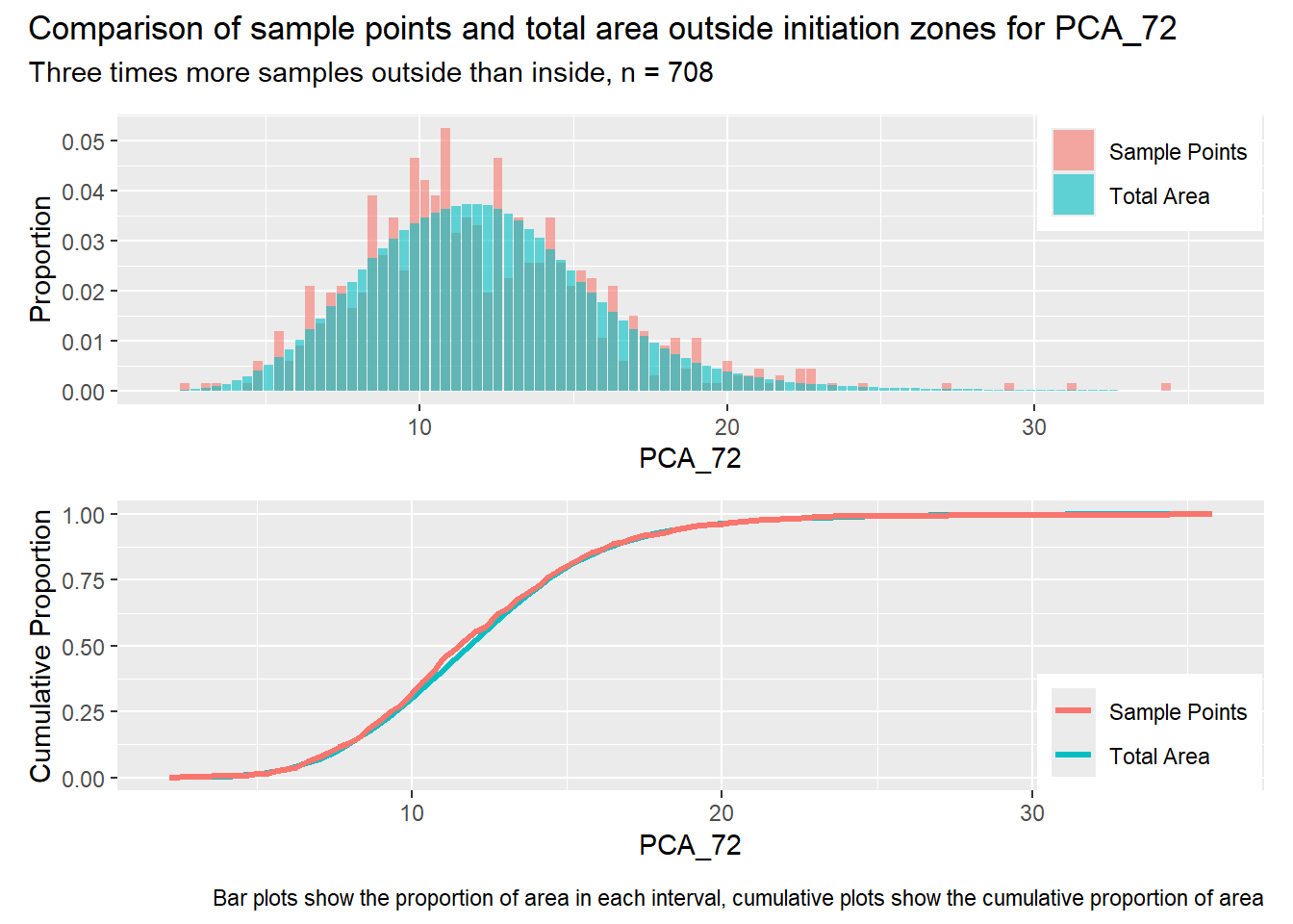
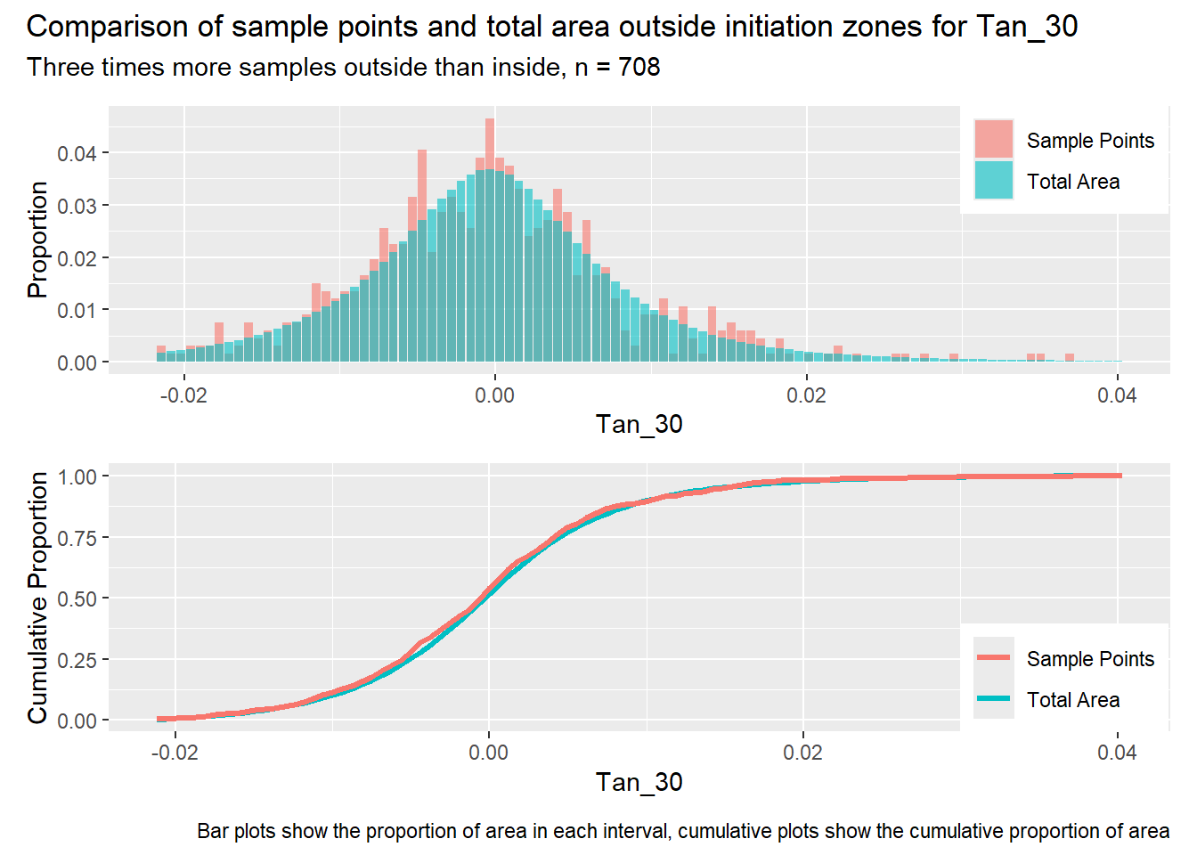
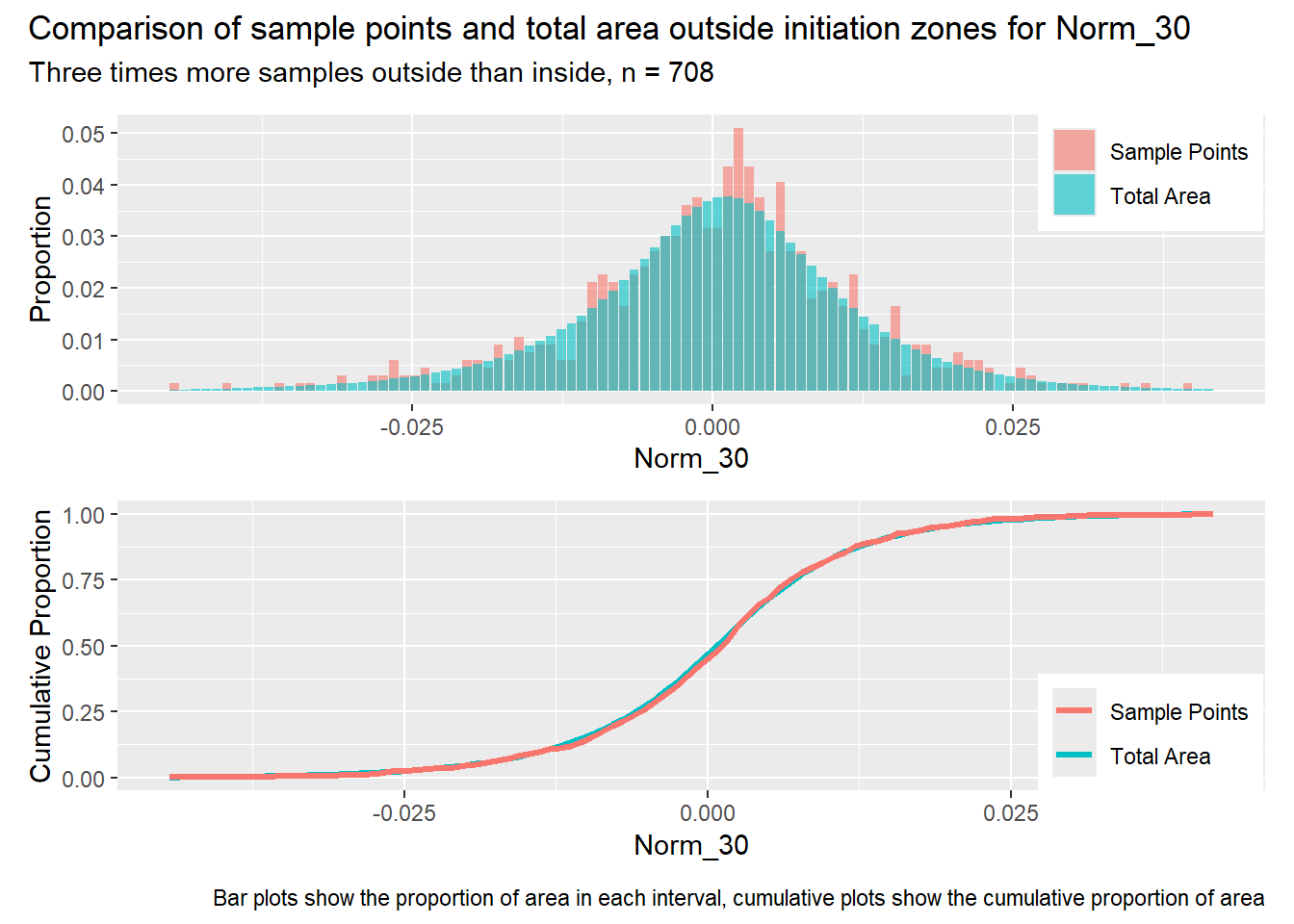
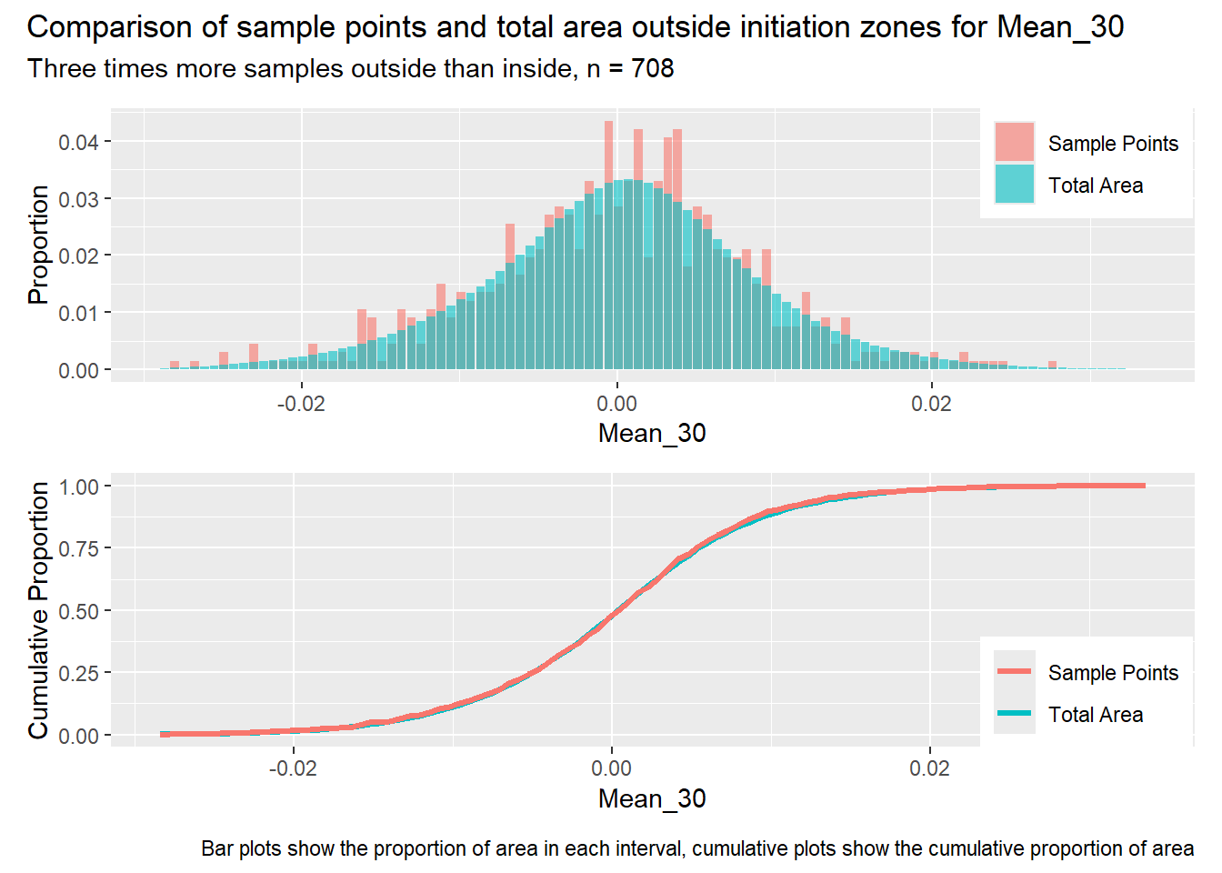
#| label: outside_1for (i in1:length(R4rasters)) { thisplot <- pbar_out[[i]] / pcum_out[[i]] thisplot <- thisplot +plot_annotation(title =paste0("Comparison of sample points and total area outside initiation zones for ", R4rasters[[i]][[1]]),subtitle ="Three times more samples outside than inside, n = 708",caption ="Bar plots show the proportion of area in each interval, cumulative plots show the cumulative proportion of area")plot(thisplot)}
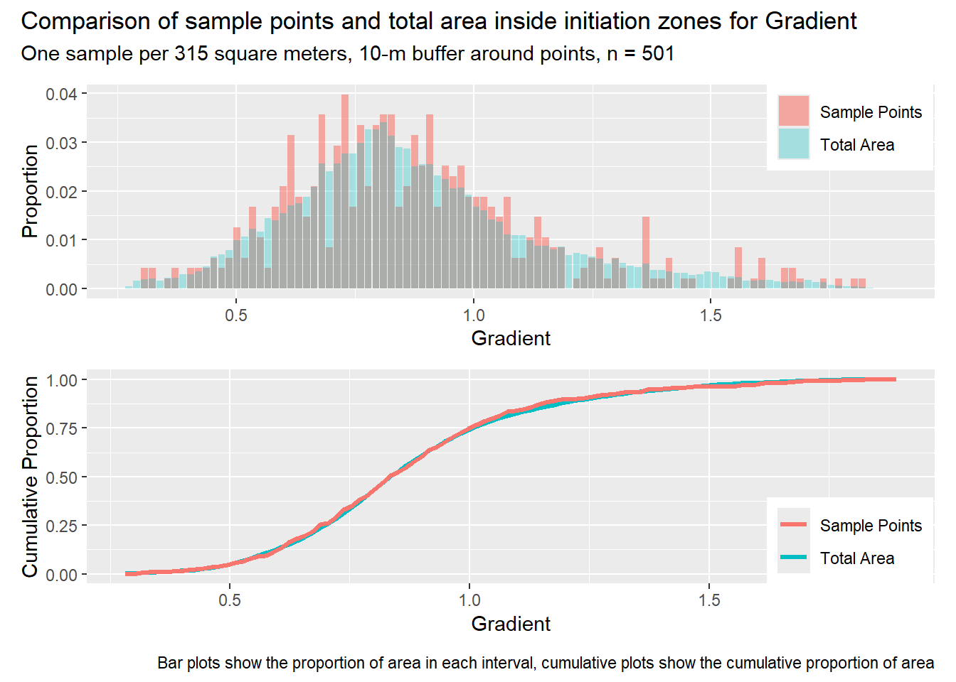
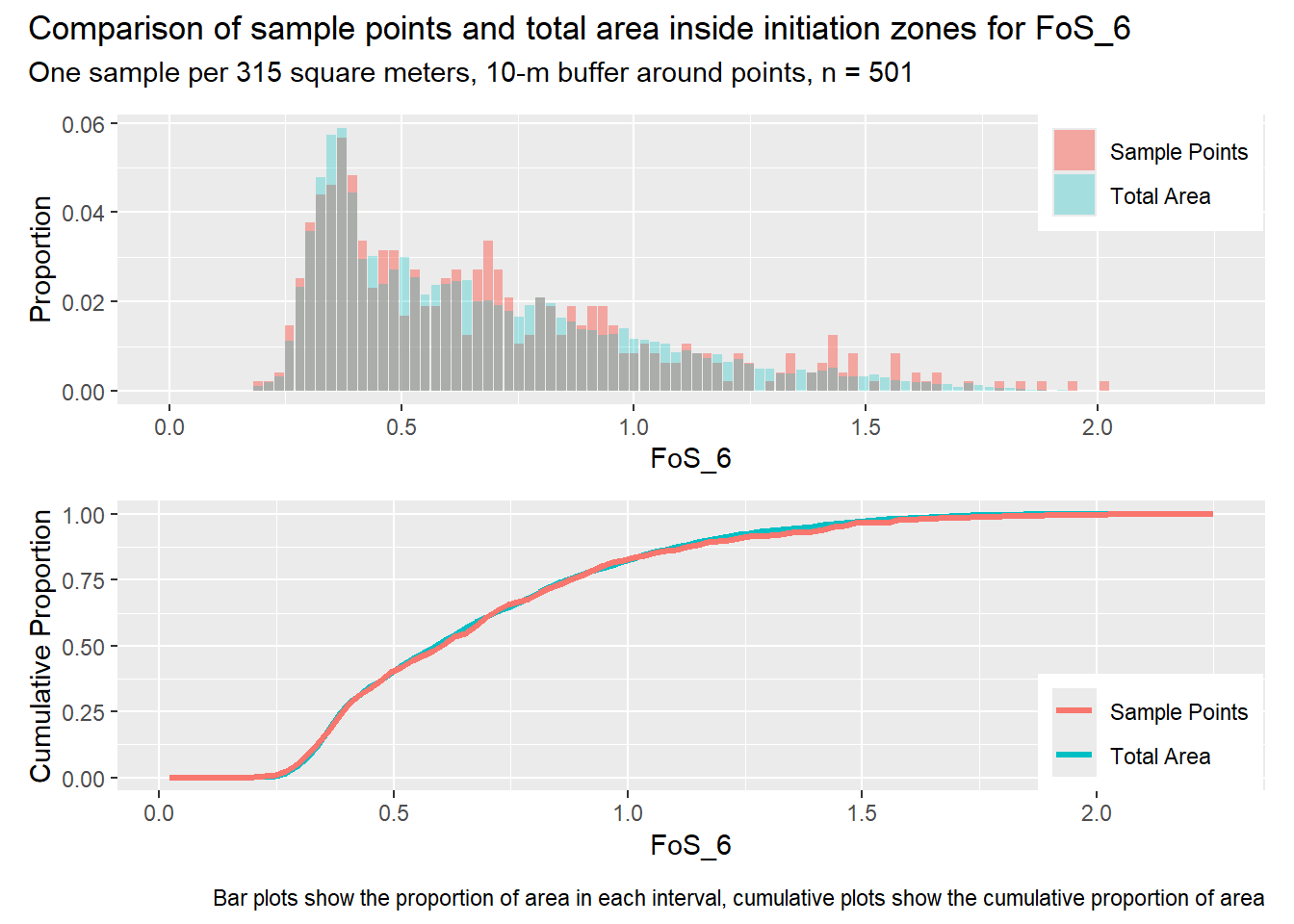
Let’s increase the density of points inside initiation zones. The previous examples had one point per initiation zone, regardless of its size. In the next example, we seek one point per every 314 m2 of initiation zone area and require a 10-m buffer around points inside the initiation zones. The spacing of points outside the initiation zones is reduced to a minimum of 100 m and we still require three times as many points outside the initiation zones as inside.
Code
# Edit input variables as neededinRaster <-"c:/work/data/wrangell/init"# initiation zones, raster created by LS_polyareaPerSample <-315.# within initiation zones, one point every areaPerSample square metersbuffer_in <-10.# buffer around sample points, in metersbuffer_out <-100.margin <-1.# margin around initiation zones to preclude sample points close to the edge, in metersratio <-3.# ratio of sample points outside initiation zones to those withinnbins <-100# number of bins for building histogramsminPatch <-100000.inPoints <-"c:/work/data/wrangell/inpoints_2"outPoints <-"c:/work/data/wrangell/outpoints_2"outMask <-"c:/work/data/wrangell/mask"outInit <-"c:/work/data/wrangell/initMod"table <-"c:/work/data/wrangell/table2"scratchDir <-"c:/work/scratch"executableDir <-"c:/work/sandbox/landslideutilities/projects/samplepoints/x64/release"returnCode <- TerrainWorksUtils::samplePoints( inRaster, areaPerSample, buffer_in, buffer_out, margin, ratio, nbins, R4rasters, I4rasters, minPatch, inPoints, outPoints, outMask, outInit, table, scratchDir, executableDir)pcum_in2 <-vector(mode ="list", length =length(R4rasters))pcum_out2 <-vector(mode ="list", length =length(R4rasters))pdif2 <-vector(mode ="list", length =length(R4rasters))pbar2 <-vector(mode ="list", length =length(R4rasters))pbar_in2 <-vector(mode ="list", length =length(R4rasters))pbar_out2 <-vector(mode ="list", length =length(R4rasters))for (i in1:length(R4rasters)) { name <- R4rasters[[i]][[1]] d_in <-as.data.table(read.csv(paste0(table, "_", name, "_in.csv"))) d_out <-as.data.table(read.csv(paste0(table, "_", name, "_out.csv"))) d_sampleIn <-as.data.table(read.csv(paste0(table,"_",name,"_inSample.csv"))) d_sampleOut <-as.data.table(read.csv(paste0(table,"_",name,"_outSample.csv"))) sum_sampleIn <- d_sampleIn[, sum(Number)] sum_sampleOut <- d_sampleOut[, sum(Number)] pbar_in2[[i]] <-ggplot() +geom_bar(data=d_sampleIn, aes(x=Mid, y=Number/sum_sampleIn, fill="Sample Points"), stat="identity", alpha=0.6) +geom_bar(data=d_in, aes(x=Mid, y=Number/sum_in, fill="Total Area"), stat="identity", alpha=0.3) +labs(x = name,y ="Proportion") +theme(legend.title =element_blank(),legend.position ="inside",legend.position.inside =c(0.9, 0.8)) pbar_out2[[i]] <-ggplot() +geom_bar(data=d_sampleOut, aes(x=Mid, y=Number/sum_sampleOut, fill="Sample Points"), stat="identity", alpha=0.6) +geom_bar(data=d_out, aes(x=Mid, y=Number/sum_out, fill="Total Area"), stat="identity", alpha=0.6) +labs(x = name,y ="Proportion") +theme(legend.title =element_blank(),legend.position ="inside",legend.position.inside =c(0.9, 0.8)) pcum_in2[[i]] <-ggplot() +geom_line(data = d_in, aes(x = Upper, y = CumulativeProp, color ="Total Area"),linewidth =1.2) +geom_line(data=d_sampleIn, aes(x=Upper, y=CumulativeProp, color="Sample Points"), linewidth=1.2) +labs(x = name,y ="Cumulative Proportion") +theme(legend.title =element_blank(),legend.position ="inside",legend.position.inside =c(0.9,0.2)) pcum_out2[[i]] <-ggplot() +geom_line(data=d_out, aes(x=Upper, y=CumulativeProp, color="Total Area"), linewidth=1.2) +geom_line(data=d_sampleOut, aes(x=Upper, y=CumulativeProp, color="Sample Points"), linewidth=1.2) +labs(x = name,y ="Cumulative Proportion") +theme(legend.title =element_blank(),legend.position ="inside",legend.position.inside =c(0.9, 0.2))}
Code
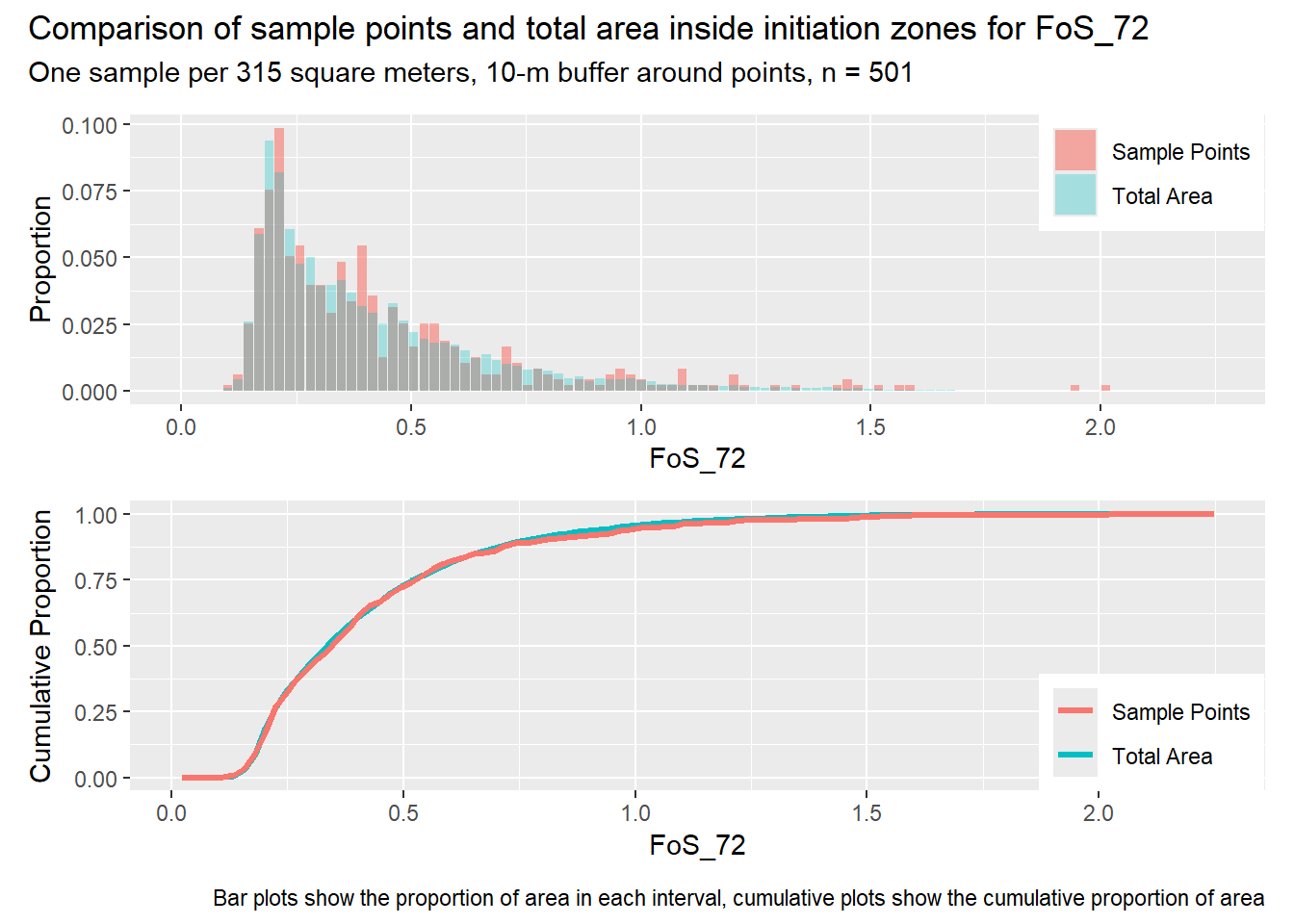
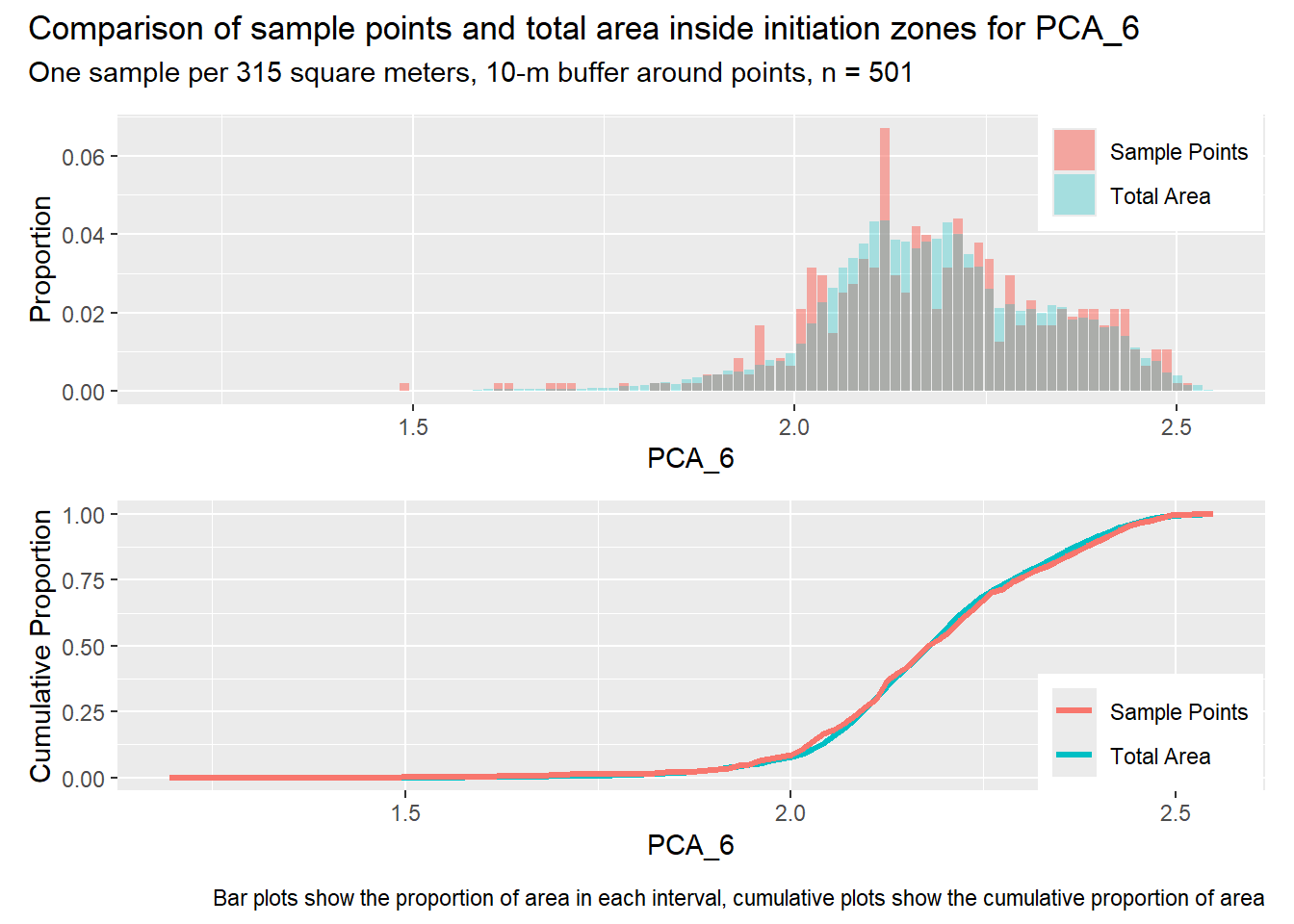
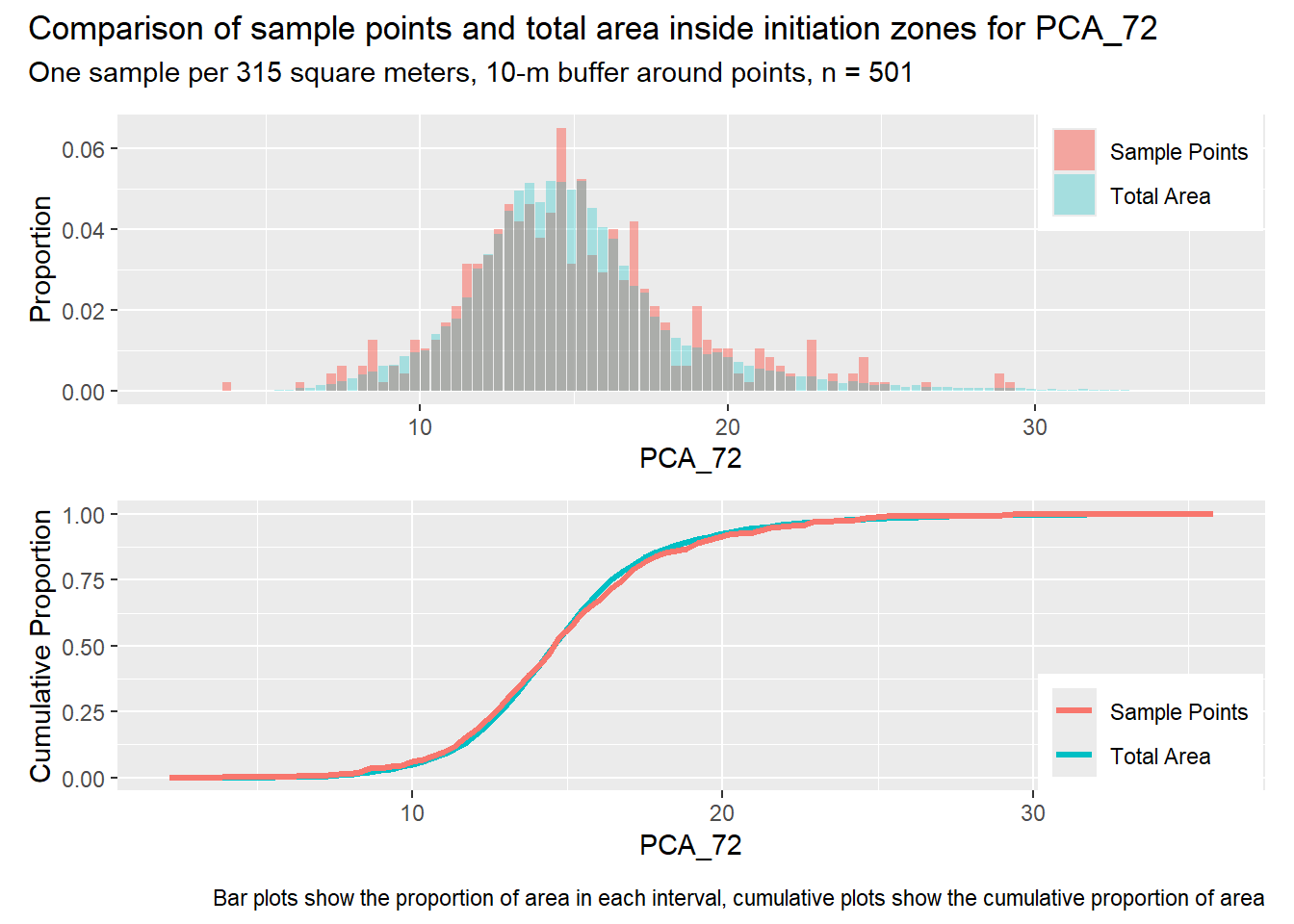
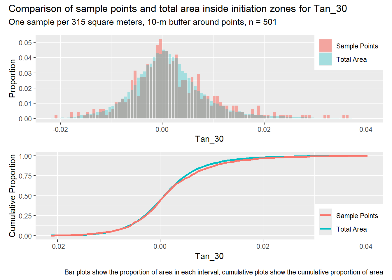
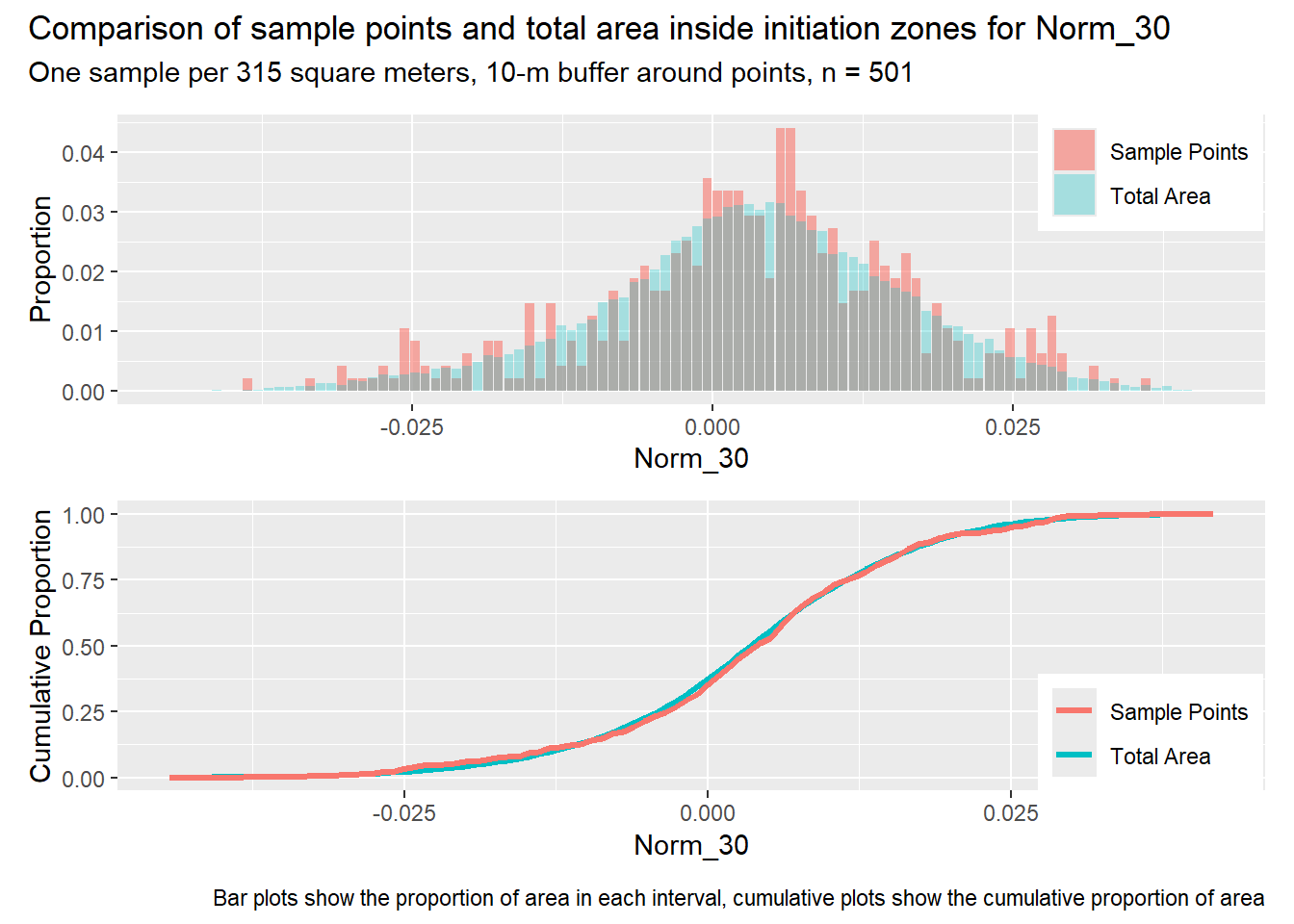
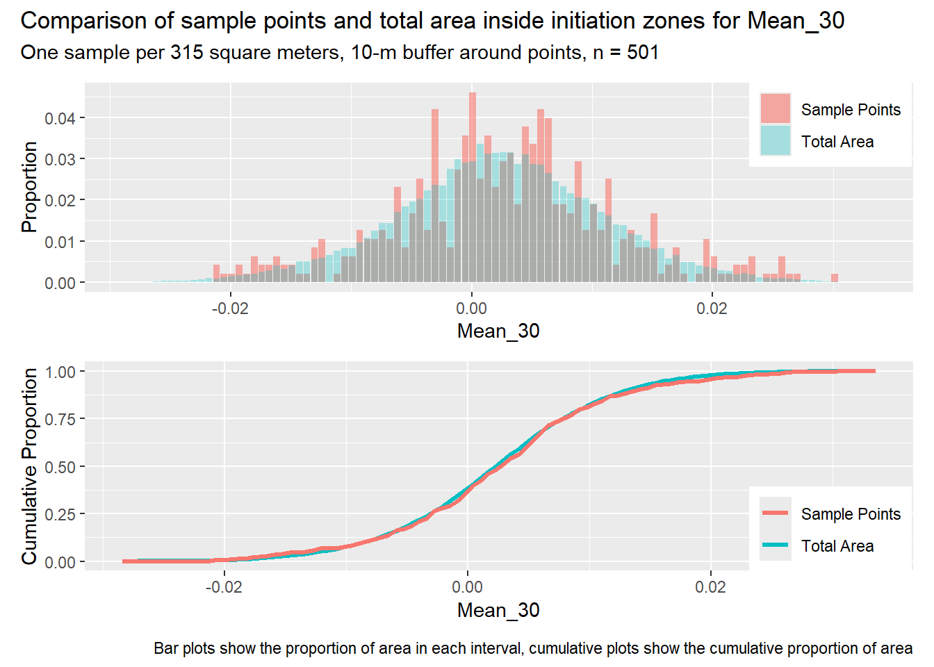
for (i in1:length(R4rasters)) { thisplot <- pbar_in2[[i]] / pcum_in2[[i]] thisplot <- thisplot +plot_annotation(title =paste0("Comparison of sample points and total area inside initiation zones for ", R4rasters[[i]][[1]]),subtitle ="One sample per 315 square meters, 10-m buffer around points, n = 501",caption ="Bar plots show the proportion of area in each interval, cumulative plots show the cumulative proportion of area")plot(thisplot)}
Code
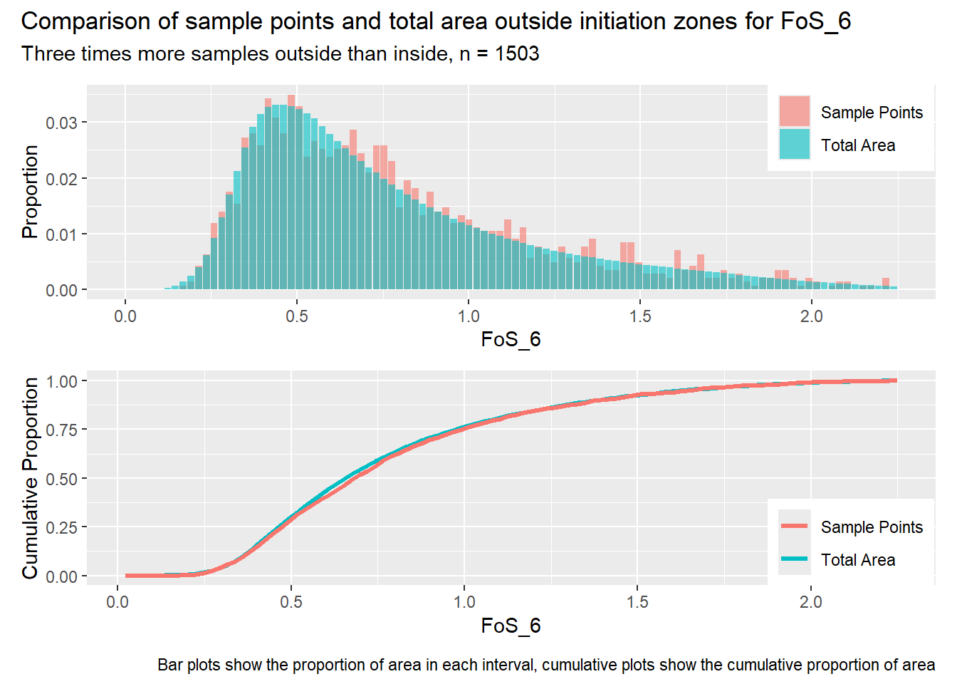
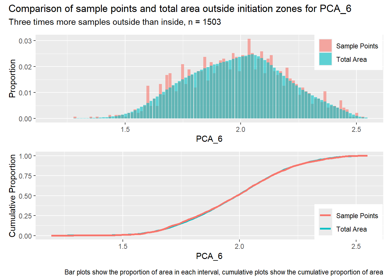
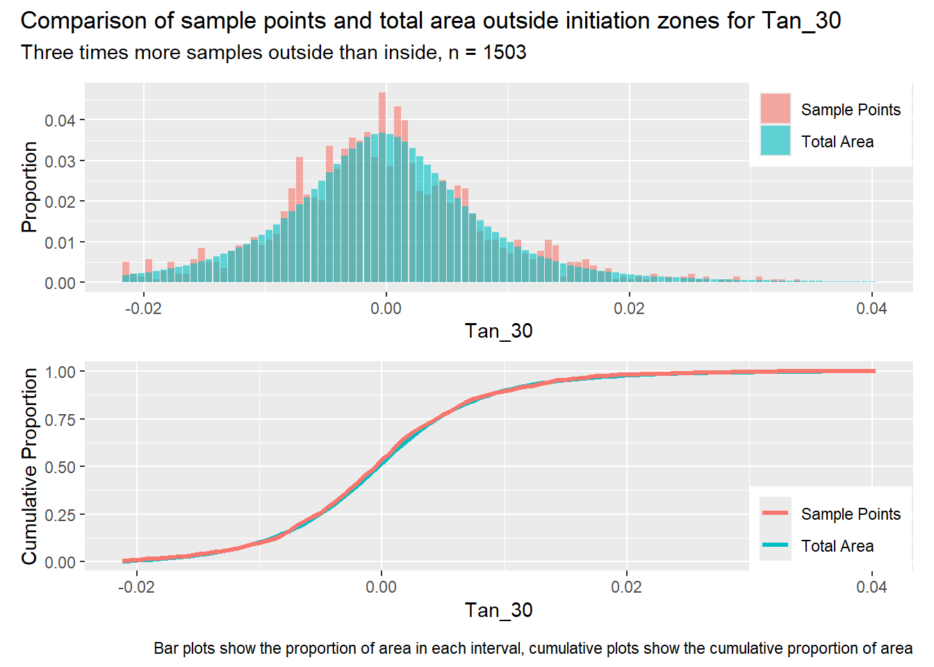
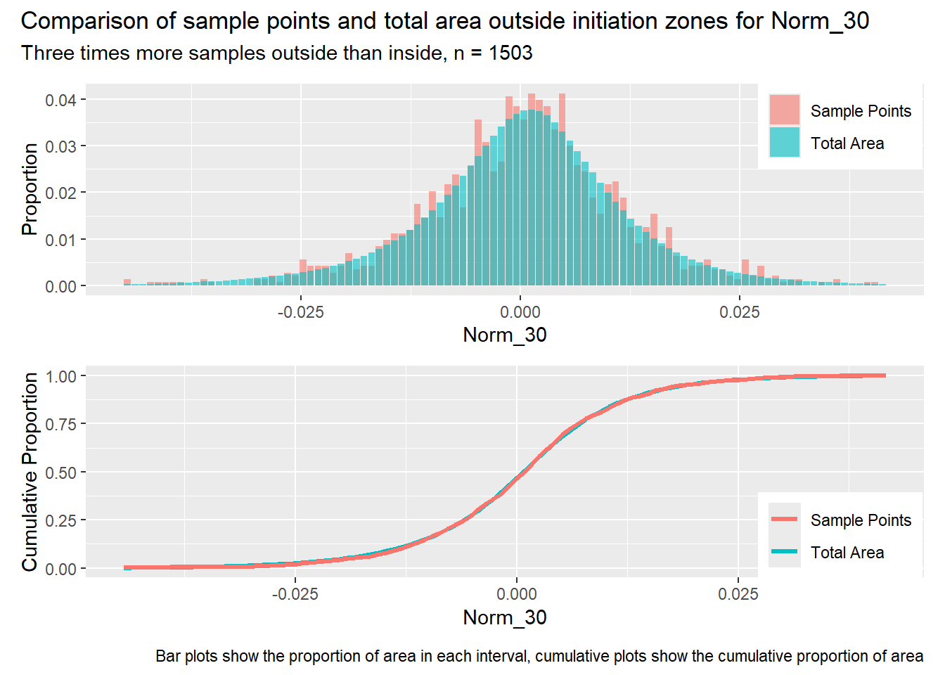
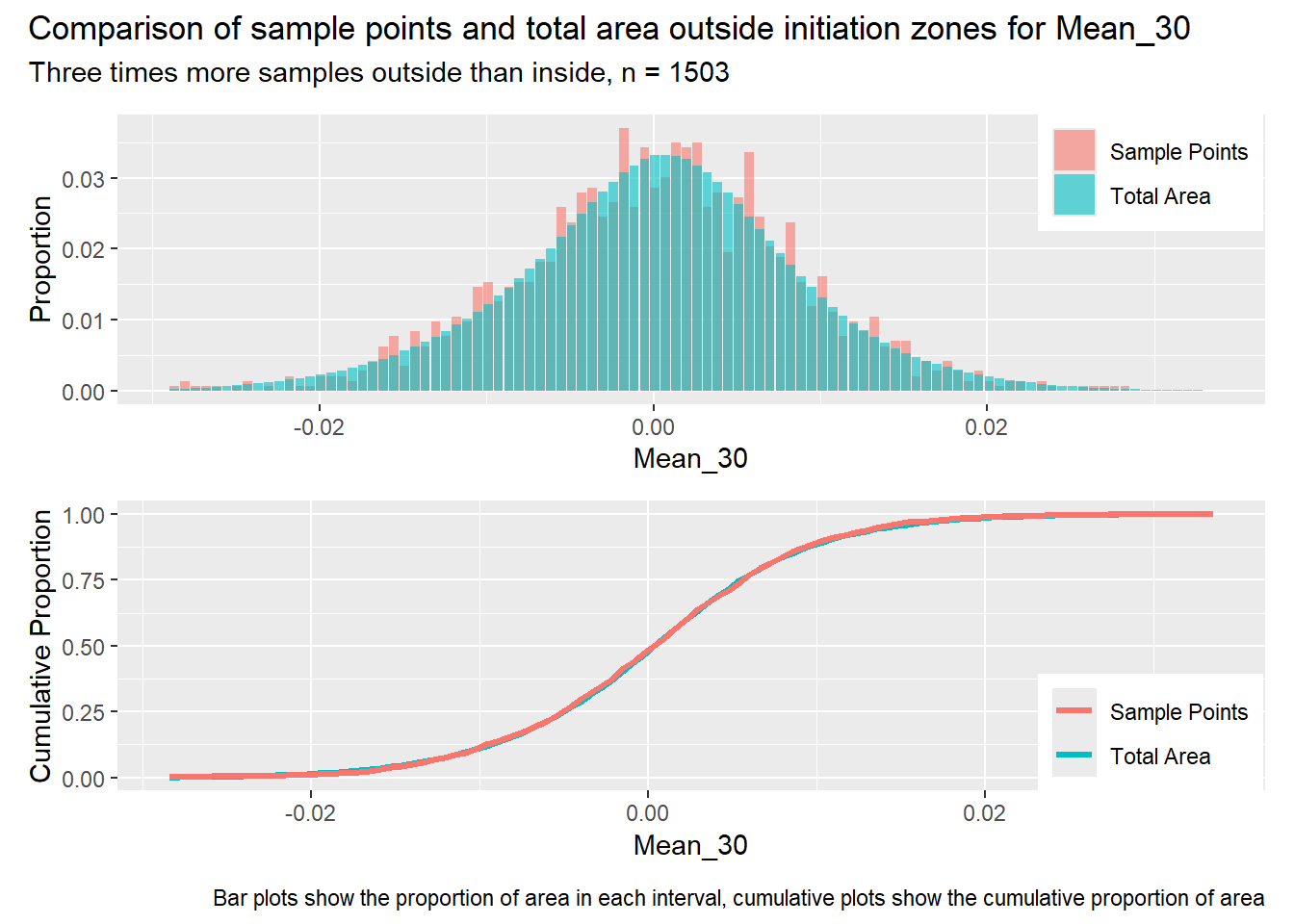
for (i in1:length(R4rasters)) { thisplot <- pbar_out2[[i]] / pcum_out2[[i]] thisplot <- thisplot +plot_annotation(title =paste0("Comparison of sample points and total area outside initiation zones for ", R4rasters[[i]][[1]]),subtitle ="Three times more samples outside than inside, n = 1503",caption ="Bar plots show the proportion of area in each interval, cumulative plots show the cumulative proportion of area")plot(thisplot)}
Increase the density of points inside the initiation zones again.
Code
# Edit input variables as neededinRaster <-"c:/work/data/wrangell/init"# initiation zones, raster created by LS_polyareaPerSample <-79.# within initiation zones, one point every areaPerSample square metersbuffer_in <-5.# buffer around sample points, in metersbuffer_out <-100.margin <-1.# margin around initiation zones to preclude sample points close to the edge, in metersratio <-3.# ratio of sample points outside initiation zones to those withinnbins <-100# number of bins for building histogramsminPatch <-100000.inPoints <-"c:/work/data/wrangell/inpoints_3"outPoints <-"c:/work/data/wrangell/outpoints_3"outMask <-"c:/work/data/wrangell/mask"outInit <-"c:/work/data/wrangell/initMod"table <-"c:/work/data/wrangell/table3"scratchDir <-"c:/work/scratch"executableDir <-"c:/work/sandbox/landslideutilities/projects/samplepoints/x64/release"returnCode <- TerrainWorksUtils::samplePoints( inRaster, areaPerSample, buffer_in, buffer_out, margin, ratio, nbins, R4rasters, I4rasters, minPatch, inPoints, outPoints, outMask, outInit, table, scratchDir, executableDir)
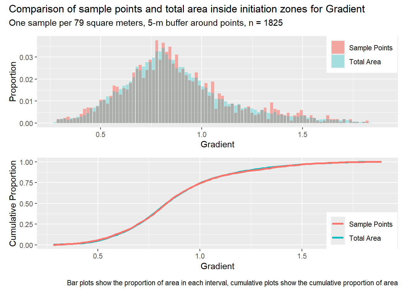
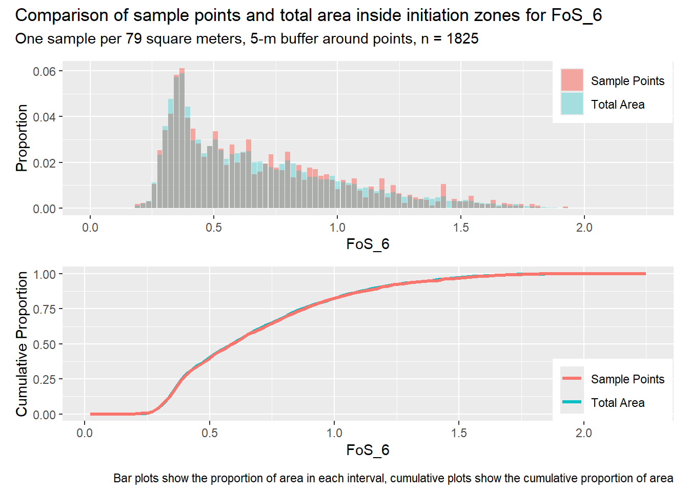
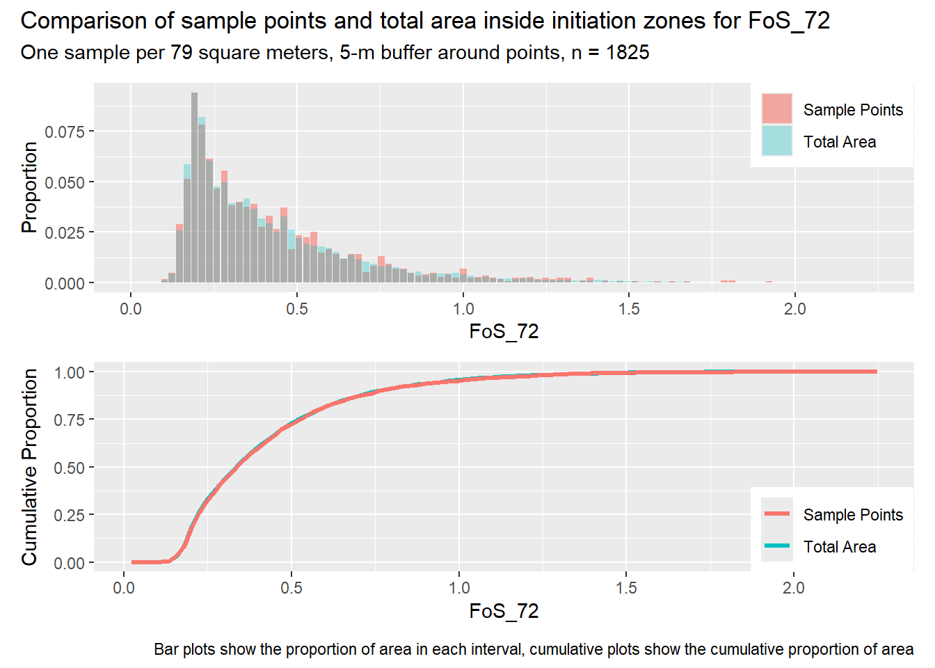
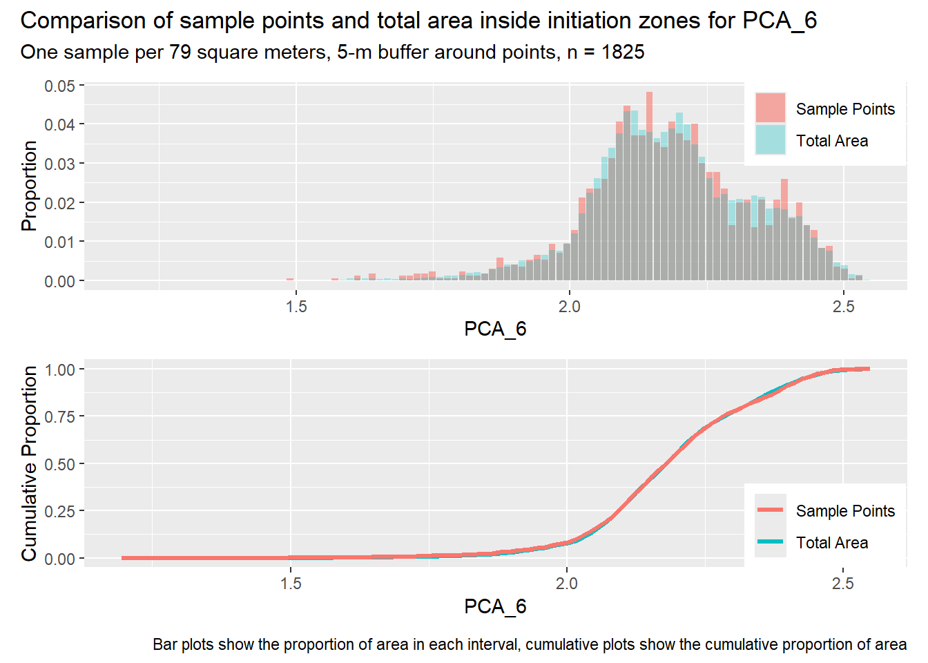
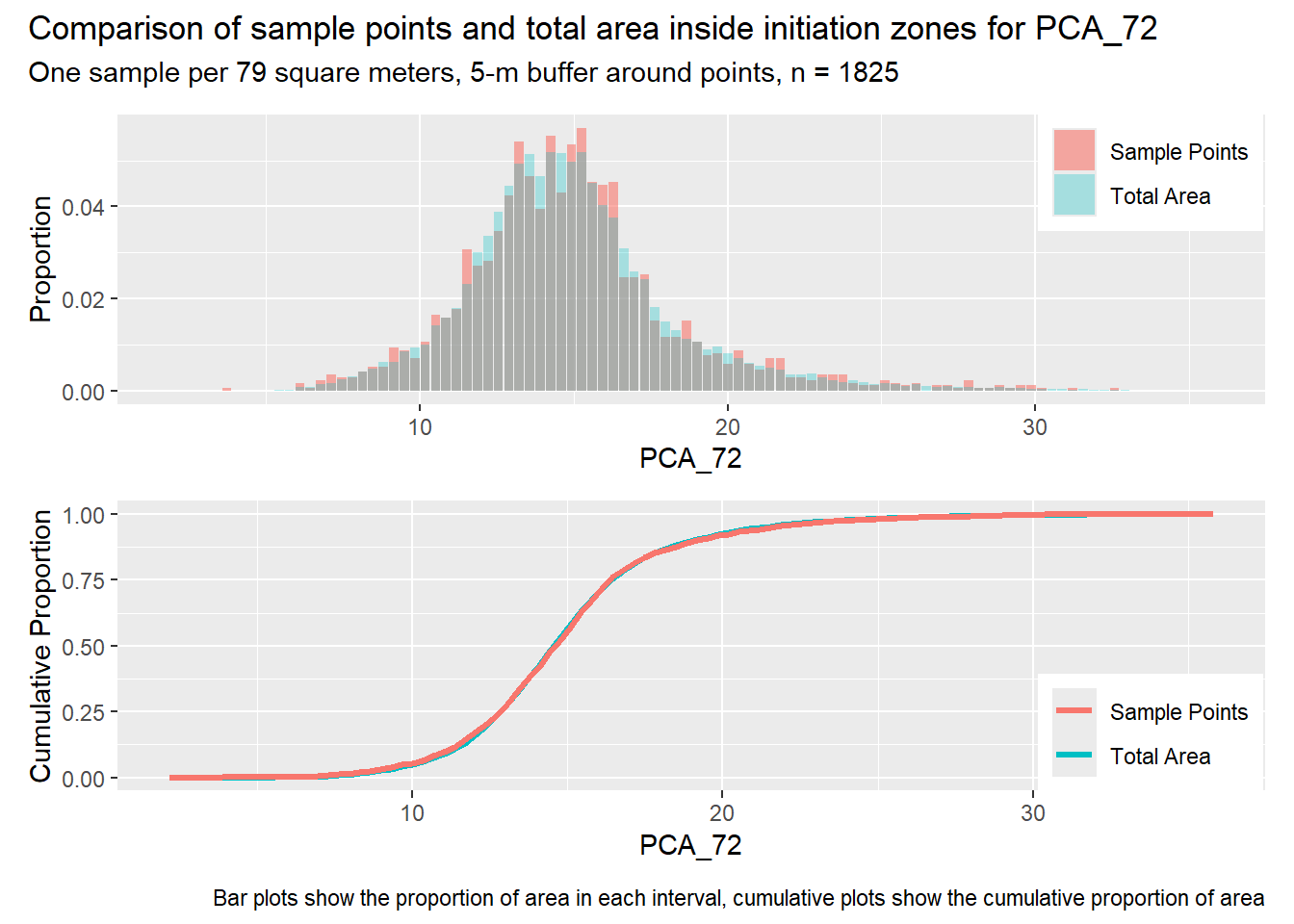
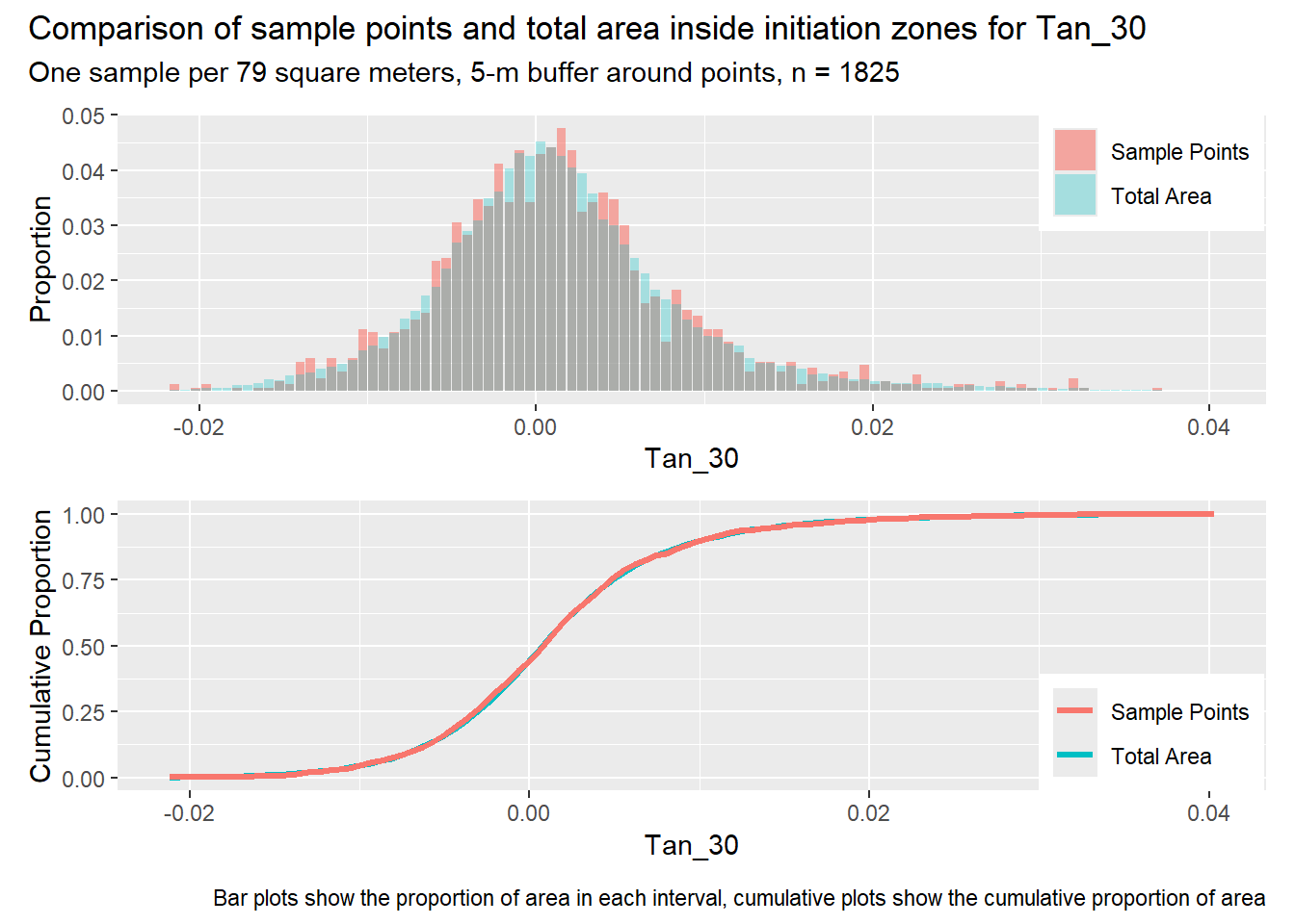
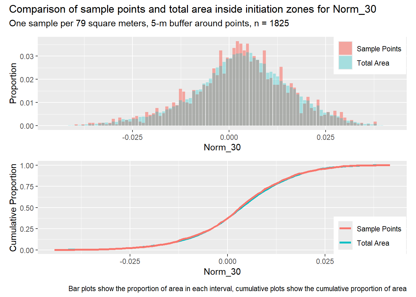
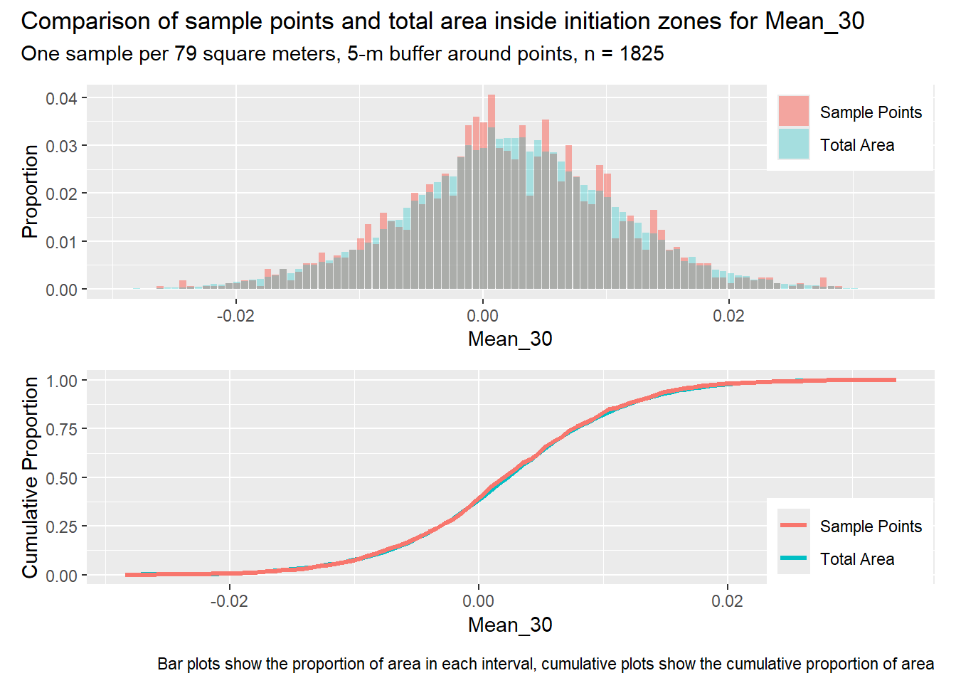
for (i in1:length(R4rasters)) { thisplot <- pbar_in3[[i]] / pcum_in3[[i]] thisplot <- thisplot +plot_annotation(title =paste0("Comparison of sample points and total area inside initiation zones for ", R4rasters[[i]][[1]]),subtitle ="One sample per 79 square meters, 5-m buffer around points, n = 1825",caption ="Bar plots show the proportion of area in each interval, cumulative plots show the cumulative proportion of area")plot(thisplot)}
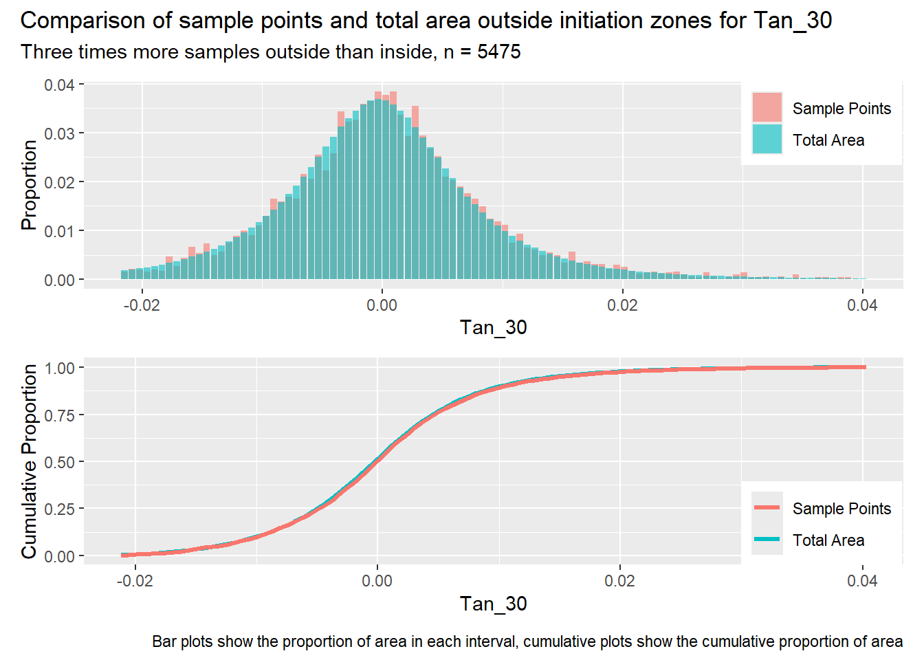
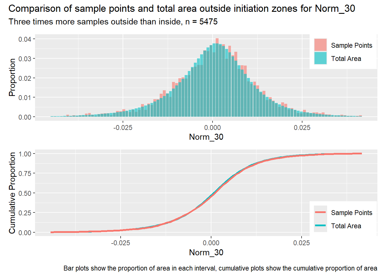
Code
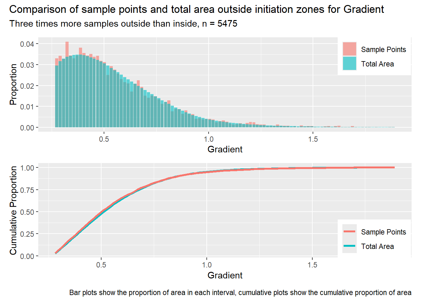
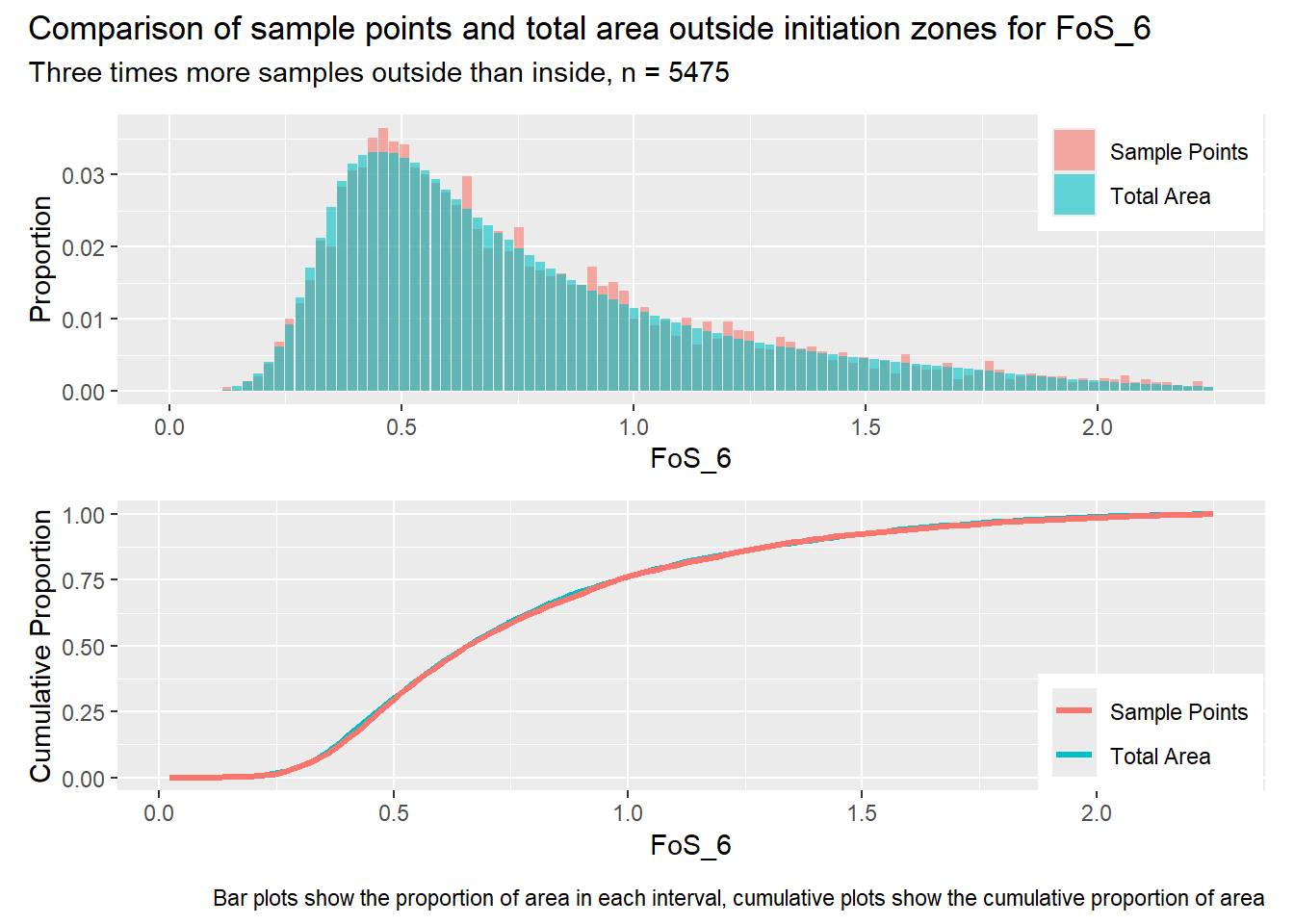
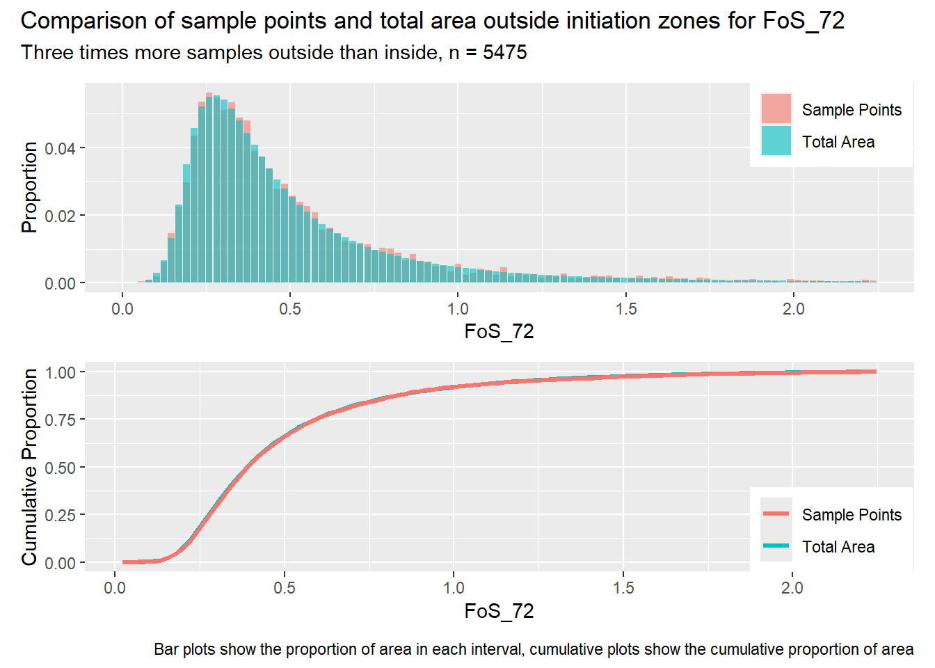
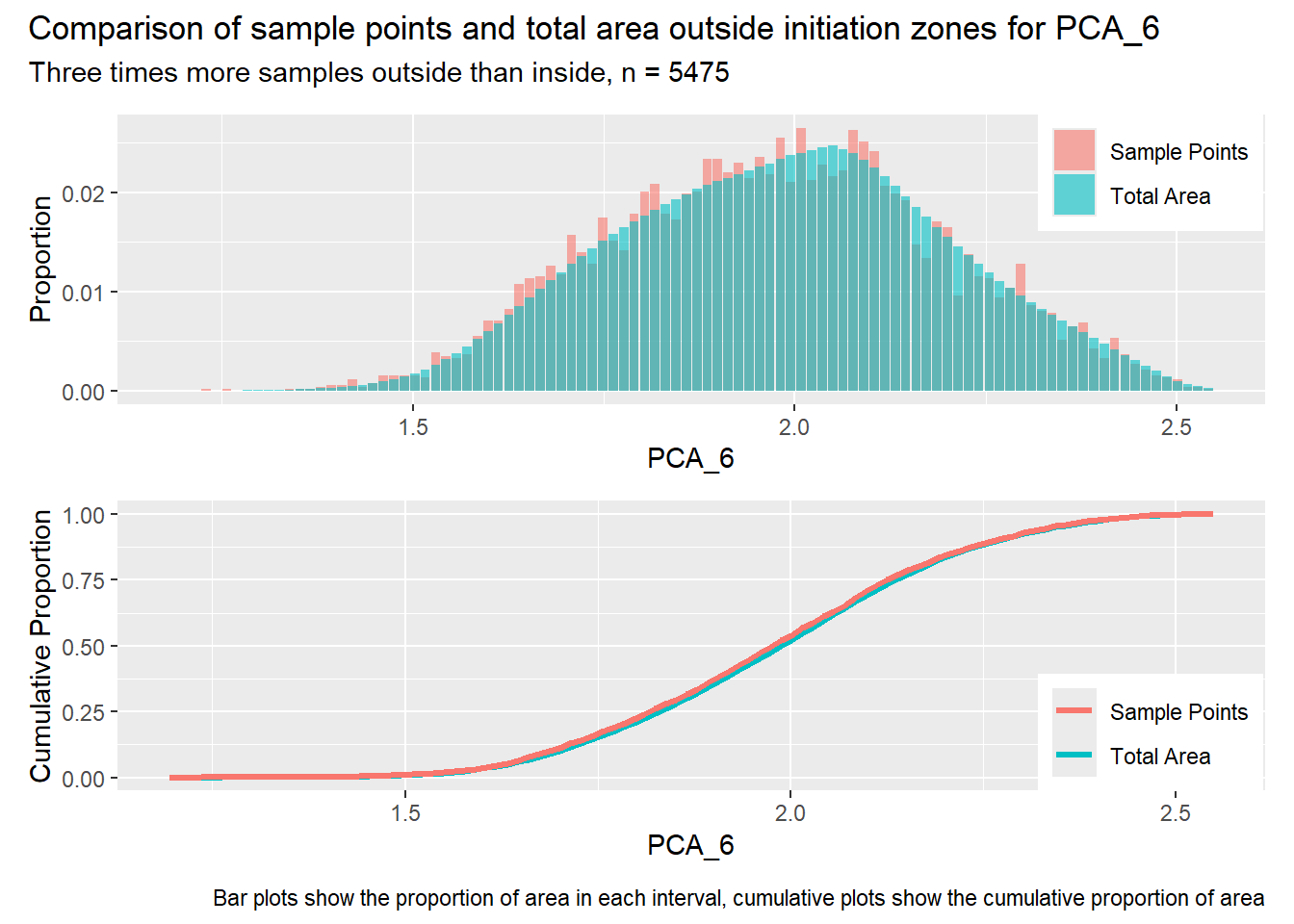
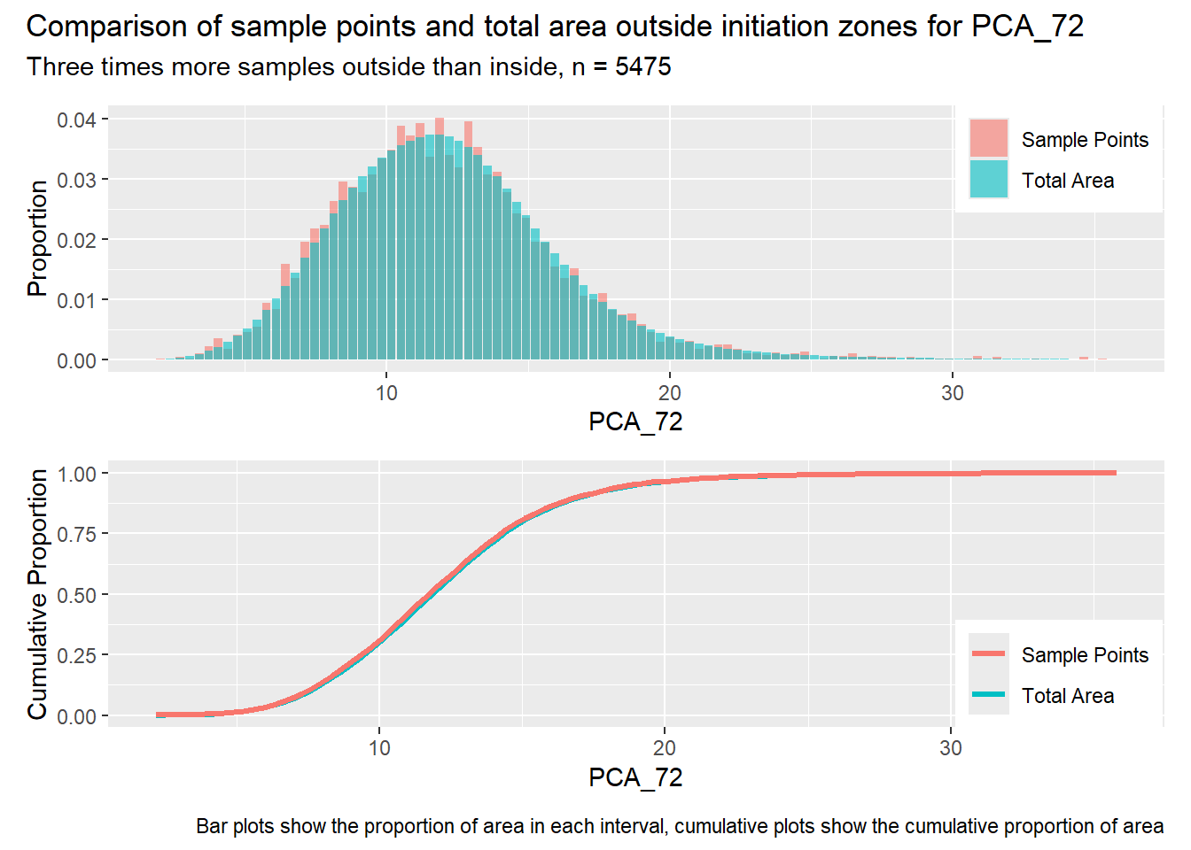
for (i in1:length(R4rasters)) { thisplot <- pbar_out3[[i]] / pcum_out3[[i]] thisplot <- thisplot +plot_annotation(title =paste0("Comparison of sample points and total area outside initiation zones for ", R4rasters[[i]][[1]]),subtitle ="Three times more samples outside than inside, n = 5475",caption ="Bar plots show the proportion of area in each interval, cumulative plots show the cumulative proportion of area")plot(thisplot)}
Each increase in the number of sample points produces an improvement in the match of the sample and total-area distributions, particularly for the initiation zones. In these examples, the initiation zones have one third as many points as the total analysis area, but they also cover only 1/1000th of the total analysis area, so the number of points per unit area in the initiation zones is about 300 times higher.
Coming:
Sampling over a multidimensional data space.
Machine-learning workflow for initiation probability.