3 Build a stream layer
It seems straightforward: define a flow direction for each DEM cell, iteratively trace flow lines downstream summing cell area as we go to create a flow accumulation raster, set a flow threshold, and voila, a stream layer. That’s basically it, but there are complications. The first two items below discuss issues that are hardwired into Chapter 1. Everything else has user-defined options, although default values are built in for most.
3.1 Flow Direction
The direction of flow for water draining out of a DEM cell is not uniquely defined. Each cell has 8 adjacent cells. Depending on the shape of the ground surface interpolated from the 9 elevation values at the midpoints of the cells, each adjacent cell may contribute all, some portion, or none of its area to the central cell and the central cell may contribute all, some portion, or none of its area (and the accumulated area of the upslope cells that flows into it) to each of the adjacent cells. The simplest strategy is to have all flow from the central cell go to one of the 8 adjacent cells. This is the “D-8” flow-direction algorithm (Jenson and Domingue 1988). It provides a poor estimate of contributing area to a cell that is biased by the 8 flow-direction options. One must also decide which of the 8 adjacent cells to direct flow to, and there are a variety of strategies for that. When D-8 flow paths are needed, we use the D8-LTD algorithm (Orlandini et al. 2003), which corrects for the directional bias. A variety of flow-direction algorithms have been developed that accommodate flow in any direction and can direct flow to multiple downslope adjacent cells (Wilson et al. 2008) and thus allow for flow dispersion. We use the D-infinity algorithm (Tarboton 1997), which allows flow into one or two adjacent cells. Flow accumulation is then calculated using the D-infinity flow directions, until the criteria for channel initiation are met. Downslope of that point, we use D-8 to prevent flow dispersion out of the channel.
3.2 Closed Depressions
These may be actual depressions with no outflow, in which case all inflowing water infiltrates to groundwater, or they be actual depressions with an outflow not visible from the DEM (e.g., road prisms with culverts), or they may be artifacts or errors in the DEM. In general, we want to define a flow path to an outlet from the DEM for every DEM cell. Even for closed depressions with no outlet, water that flows into them exits through some groundwater flow path and eventually flows to a stream somewhere downslope or out of the area represented with the DEM. Two primary approaches are used to deal with closed depressions (Wang, Qin, and Zhu 2019).
3.2.1 Fillling
This is the simplest. The depression is filled to the elevation of its lowest pour point (where water would spill out if the depression were filled). Flow directions through the closed depression are then directed toward the pour point. This option destroys any information about flow directions within the closed depression, which we would rather avoid.
3.2.2 Carving
A path is carved from the depression pour point to the lowest point in the depression and from to a location along the flow path from the pour point where the elevation becomes less than or equal to the lowest point in the depression. Flow within the depression is then directed to the lowest point and then out of the depression along the carved path (Soille, Vogt, and Colombo 2003). The flow paths from the pour point heading into and away from the depression follow D8-LTD flow directions. This is the preferred option and the one used in bldgrds.
3.3 Channel initiation
We need to specify the conditions where channels initiate. This determines the upslope extent of the channel network and the channel density. We have several strategies:
3.3.1 Local topographic position
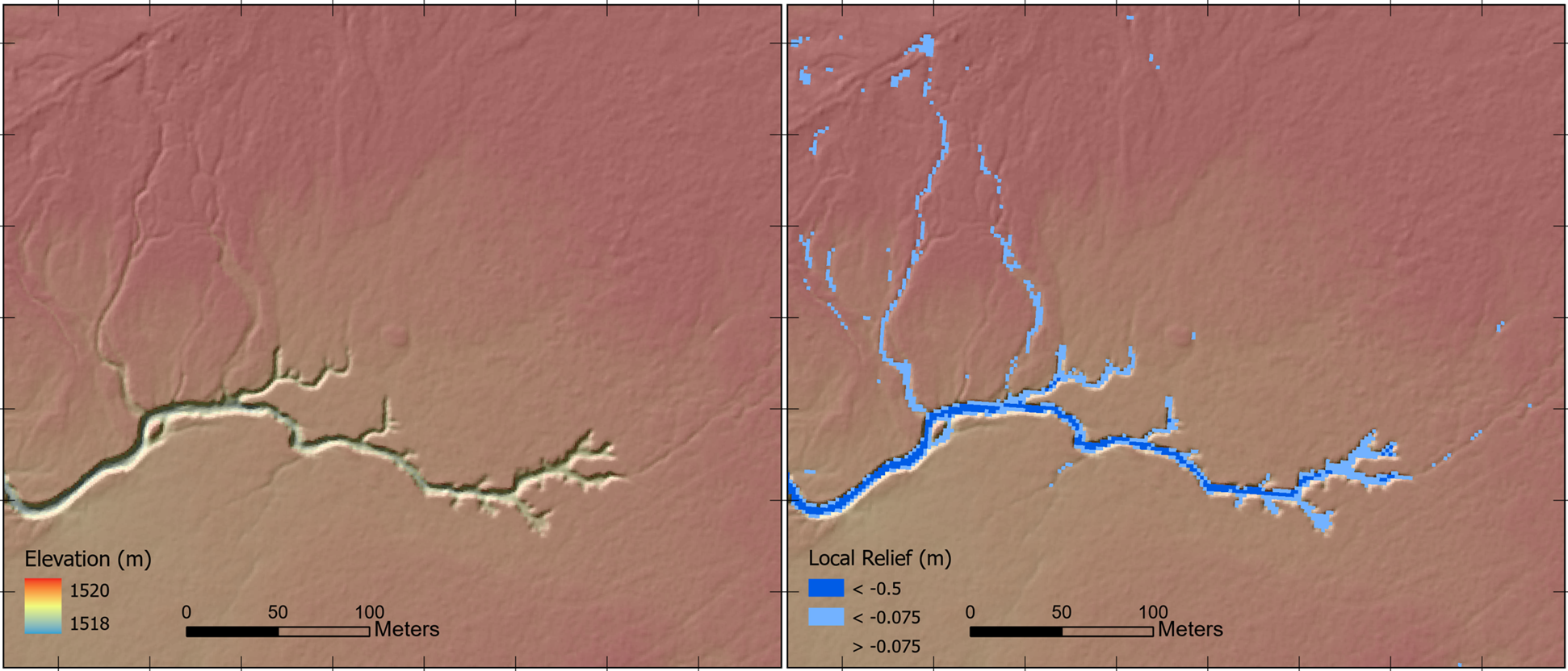
For high-resolution DEMs interpolated from high-density ground returns (e.g., >1/m2), channels are visible directly in the DEM, as shown in Figure 3.1 below. Channels can be highlighted using a measure of local topographic position (LTP), which provides an indicator of the elevation of a DEM grid point relative to its neighbors. Absolute LTP measures give the difference in elevation of the grid point compared to the mean or median grid-point elevations within a specified circular neighborhood. Relative measures normalize that elevation difference by some measure of elevation variability in the neighborhood. Deviation from mean elevation (DEV), for example, divides the difference from mean elevation by the standard deviation of DEM grid-point elevations within the neighborhood (Newman, Lindsay, and Cockburn 2018). Thus, a small channel incised 0.25 meters traversing flat, low-relief terrain (with a small standard deviation in elevation values) will have a large DEV value compared to a small channel incised 0.25 meters traversing steep, rough terrain (with a larger standard deviation). For determining upslope channel extent, we can specify an LTP threshold value and exclude channel initiation in areas where the LTP value is greater than that threshold (i.e., channel incision is too small). One must decide on whether to use an absolute or relative measure and on the appropriate length scale for the local neighborhood. I find an absolute measure easier to interpret than a relative measure, because it provides a direct estimate of the depth of channel incision; I can decide that traced channels begin only when a channel is incised to more than 0.2 meters (LTP < -0.2), for example. The radius to choose for the local neighborhood should be set relative to the resolution of the DEM, the roughness of the terrain (greater roughness requires larger neighborhoods), and the smallest width of channels you want to identify. Typically, at their upslope extent, channels are less than a meter wide, so a radius of five meters or more will suffice for calculating LTP.
3.3.2 Area-slope threshold
Where the lidar ground-return-point density is insufficient to resolve channels at their upslope extent, we need to infer channel-initiation locations indirectly. One strategy for this is to estimate where on the landscape there may be sufficient flowing water to erode a channel. The contributing (drainage) area to any point on the landscape indicates the upslope area from which overland flow and water infiltrating to shallow subsurface flow through the soil can originate. Hence, differences in contributing area provide indicators of relative differences in overland- and shallow-subsurface discharge; greater contributing area implies greater discharge. This is the idea behind using thresholds in contributing area to estimate upslope channel extent: for a given climate and terrain, some minimum contributing area is required for sufficient discharge to erode a channel. The erosive power of water depends not only on how much water there is, but also on the steepness of the slope it is flowing over or through. Hence, threshold values for functions of contributing area and ground-surface slope may provide better indicators of where channels initiate than contributing area alone. We use the function ASe, where A is contributing area, S is tangent of the ground-surface gradient, and e is a user-specified exponent (Montgomery and Foufoula-Georgiou 1993). Contributing area may be specified as specific contributing area, which is the contributing area divided by the length of a contour line crossed by flow exiting the DEM cell (Gallant and Hutchinson 2011). This accounts for effects of topographic convergence and divergence on the depth of flow and is the default in bldgrds.
Basin topography is found to exhibit certain scaling relationships between contributing area and gradient that delineate divergent, convergent, and channelized topography (Ijjasz-Vasquez and Bras 1995). We capitalize on these to calibrate threshold values for channel initiation. Following Clarke, Burnett, and Miller (2008), we plot channel density as a function of the ASe value and look for the inflection in log-log plots that indicate a transition to the channelized regime, as shown in Figure 3.2 below. With the “CALIBRATE” keyword, bldgrds will generate an output comma delimited file (.csv) with which to construct this graph.
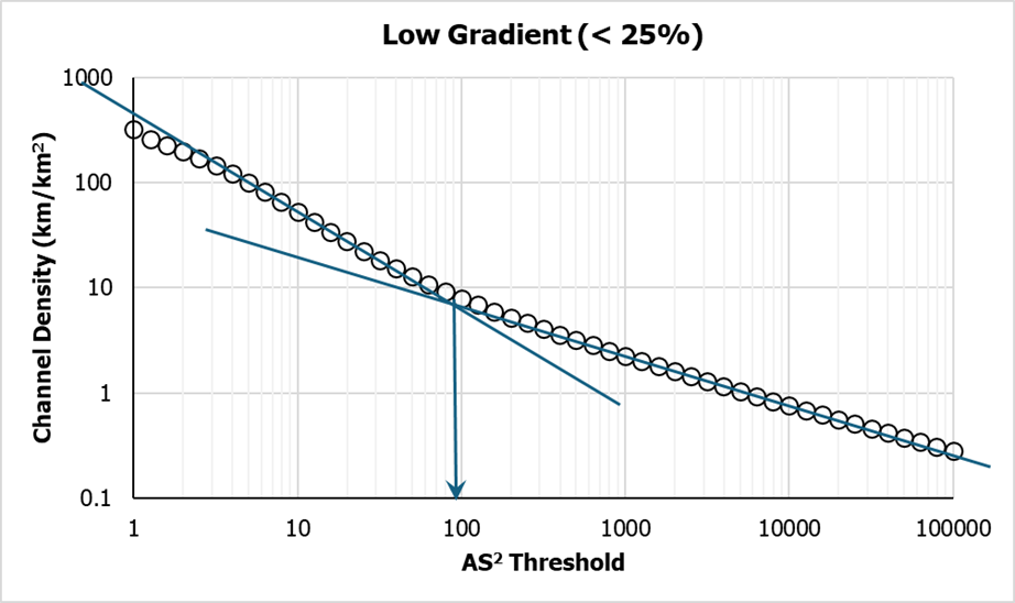
This provides a ball-park estimate of the threshold value appropriate for the terrain as represented with the DEM. Plots are produced separately for steep terrain and low-gradient terrain, under the assumption that channel-forming processes may differ, e.g., landsliding on steep terrain and fluvial erosion on low-gradient terrain.
3.3.3 Plan curvature
Plan curvature measures the rate of change in elevation measured in a direction tangent to a contour line; it indicates the curvature of the contour. Tangential curvature is similar, but measures the rate of change relative to a plane oriented tangent to the ground surface, whereas plan curvature measures curvature relative to a horizontal plane (Minár, Evans, and Jenčo 2020). Both provide another measure for topographic indication of presence of a channel. Bldgrds has the option to specify thresholds of plan (or tangential) curvature for channel initiation. These thresholds can be determined by building curvature rasters using the makegrids program, classifying by proposed threshold values, and plotting on a shaded relief image to see where a proposed threshold would allow channel initiation. The LTP thresholds described above provide a similar and more easily interpreted method of using topography inferred from the DEM for identifying channels.
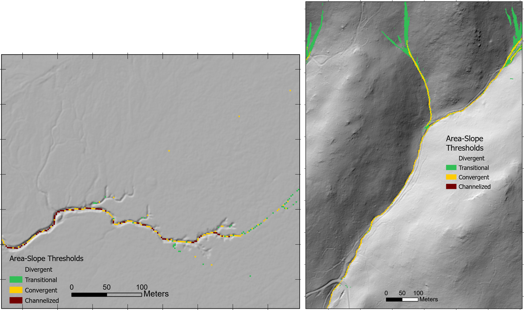
3.3.4 Minimum flow length
Bldgrds iteratively traverses every flow path within a DEM in a downslope direction and checks each cell to see if it meets the channel-initiation criteria. As seen in the Figure 3.1 and Figure 3.3 above, the criteria can be met for some portion of the flow path, but then no longer be met further downslope. Bldgrds requires specification of the minimum length over which the initiation criteria must be met before it will initialize a channel. The appropriate length depends on the resolution of the DEM and on the roughness of the terrain. If topographic channel indicators are indistinct, small zones where initiation thresholds are met can arise from noise in the DEM or small-scale roughness in the terrain.
3.4 Channel Courses
The cell-to-cell D8 flow paths used once channel initiation is met do not always follow the same course that the actual channels do. Sometimes evidence of the channel flow path is not visible in the DEM, sometimes there are multiple options, sometimes noise in the DEM misdirects the flow path. It can help to use information from DEM cells beyond those immediately adjacent and to bring in information from other data sources. Here are options used by bldgrds.
3.4.1 Flow indicators
Topographic indicators of a channel can also be used to guide channelized flow paths. The flowcat program (for flow categorization) uses one to four such indicators: 1) a threshold in flow accumulation calculated with D-infinity flow directions and no channel initiation, 2) geomorphon valley and pit types Jasiewicz and Stepinski (2013), 3) a threshold in plan (or tangential) curvature, and 4) a threshold for deviation from mean elevation (DEV). FlowCat creates a raster with each cell indicating the number of specified flow indicators that are met at each DEM cell. If all four indicators are used, then raster values range from 0 to 4. Bldgrds preferentially directs channels towards raster-cell values greater than zero, or greater than a specified minimum (e.g., if all four indicators are used, a minimum of two indicators must be met). This is done by excavating the corresponding cells in the DEM by a multiple of the flow-indicator raster.
3.4.2 Water mask
Infrared laser signals are largely absorbed by water and suffer from specular reflections, so there are few or no signal returns from open water, as illustrated in Figure 3.4 below.
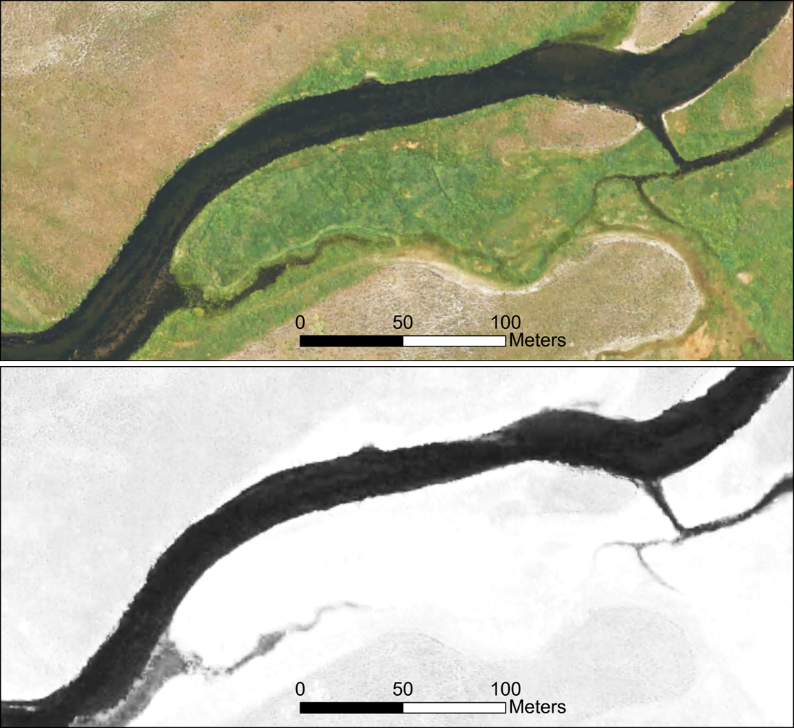
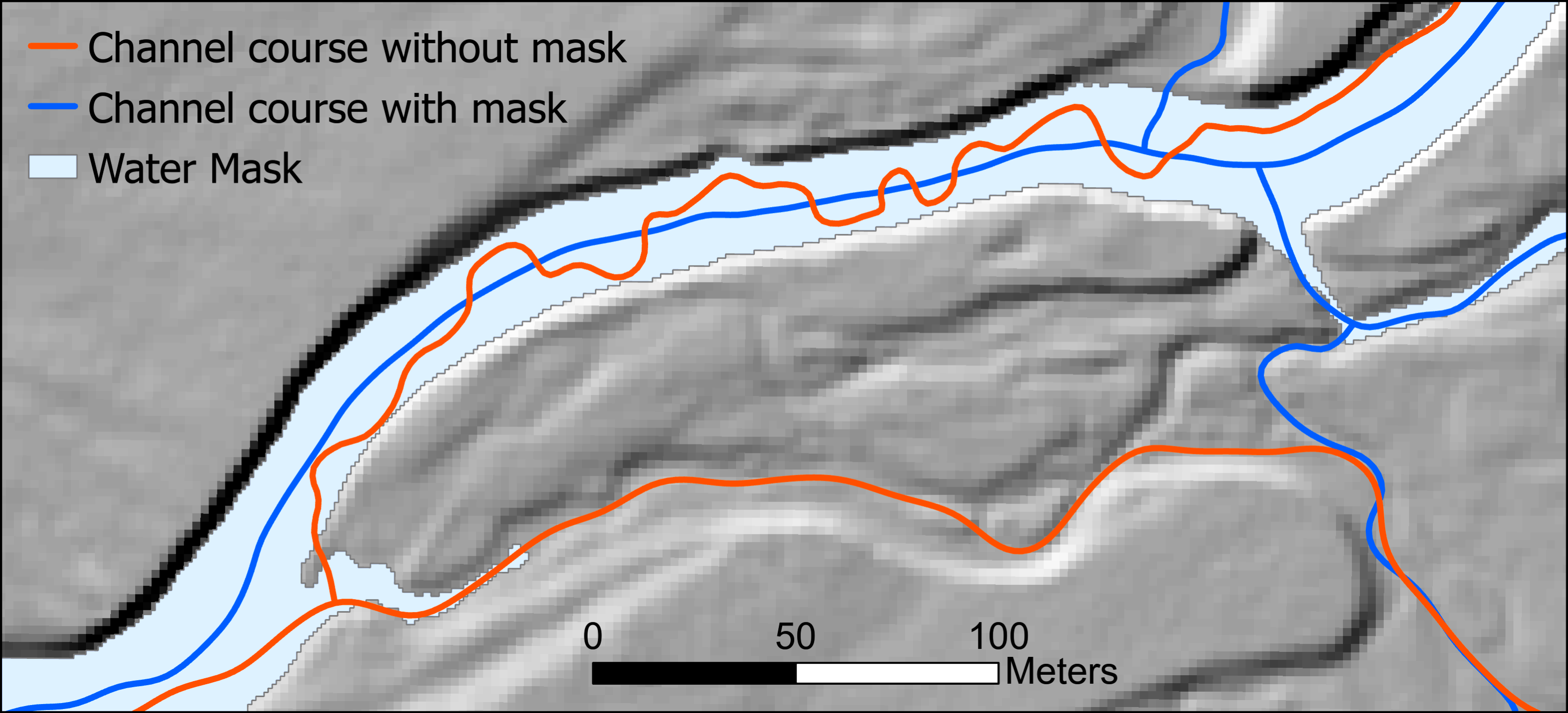
Lidar DEMs often have areas of water “hydroflattened”, so that the open-water zone has a single uniform elevation or a uniformly downstream decreasing elevation. In other cases, elevations over the open-water zone are interpolated from ground returns on either side, which can generate noisy DEM elevation values through the zone of open water. This can result in zig-zaggy flow paths, as shown in Figure 3.5 below, which then overestimate channel length and affect values of corresponding derivatives, such as channel gradient.
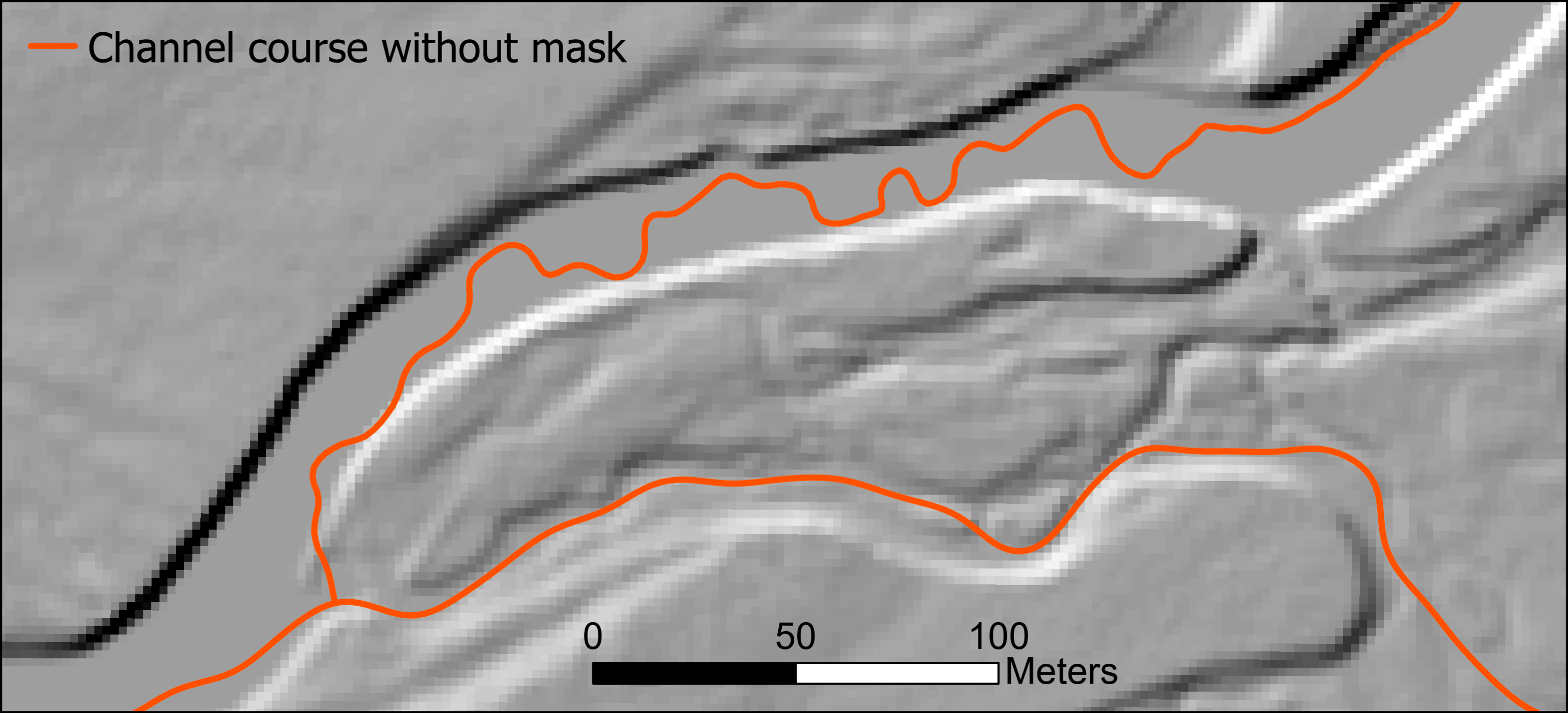
We want channel flow paths through zones of open water to be smooth and to track through the center of the open-water zone. To accomplish that, we can provide bldgrds with a separate raster or polygonal water-mask layer. Bldgrds will direct flow paths through the center of these zones.
In some cases, breaklines for hydroflattening are provided with lidar-derived DEMs. In other cases, we can build a water mask using multi-band imagery, like that shown in @fig-RGB_Infrared above. Open water appears dark in infra-red bands and can be delineated using image segmentation. Program waterMaskByTopo can generate a water-mask raster using the infrared band from e.g., NAIP. It also uses thresholds in DEV (Deviation from Mean Elevation, a Topographic Position Index) and gradient to distinguish shadows.
3.4.3 DEM derivatives
Azimuth, plan curvature, and the direction of steepest descent can also be used with varying degrees of influence to guide channelized flow directions. Azimuth and plan curvature are measured over a specified length scale. By specifying a length greater than the DEM grid-point spacing, azimuth and curvature use information beyond the elevation of adjacent points, which can reduce the influence of noise in the DEM. It can also cause flow paths to deviate from the steepest-descent path to an adjacent cell. One or more of these indicators may be used and, if more than one are specified, different degrees of influence can be specified for each. The choice of indicators, of length scales, and of the degree of influence to specify requires iterative experimentation.
3.5 Flow diversions
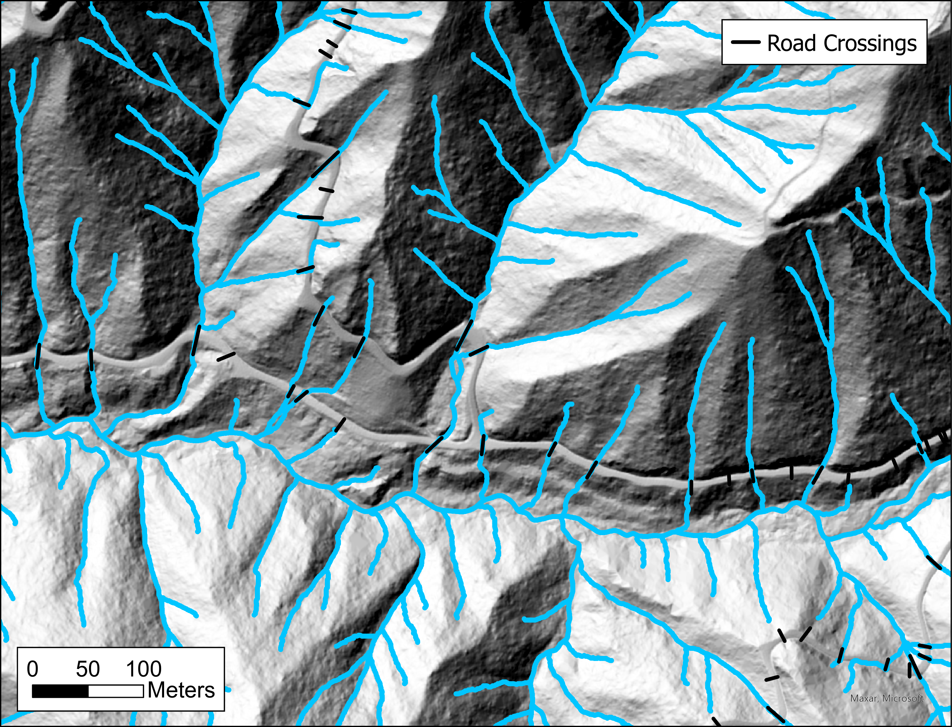
High-resolution lidar DEMs resolve road prisms and other potential blockages to channel flow. The carving algorithm used to drain closed depressions will often trace the correct flow path, but not in all cases, as shown in Figure 3.7 below. If these apparent blockages have drainage structures, such as culverts, not visible in the DEM, these need to be specified from other data sources.
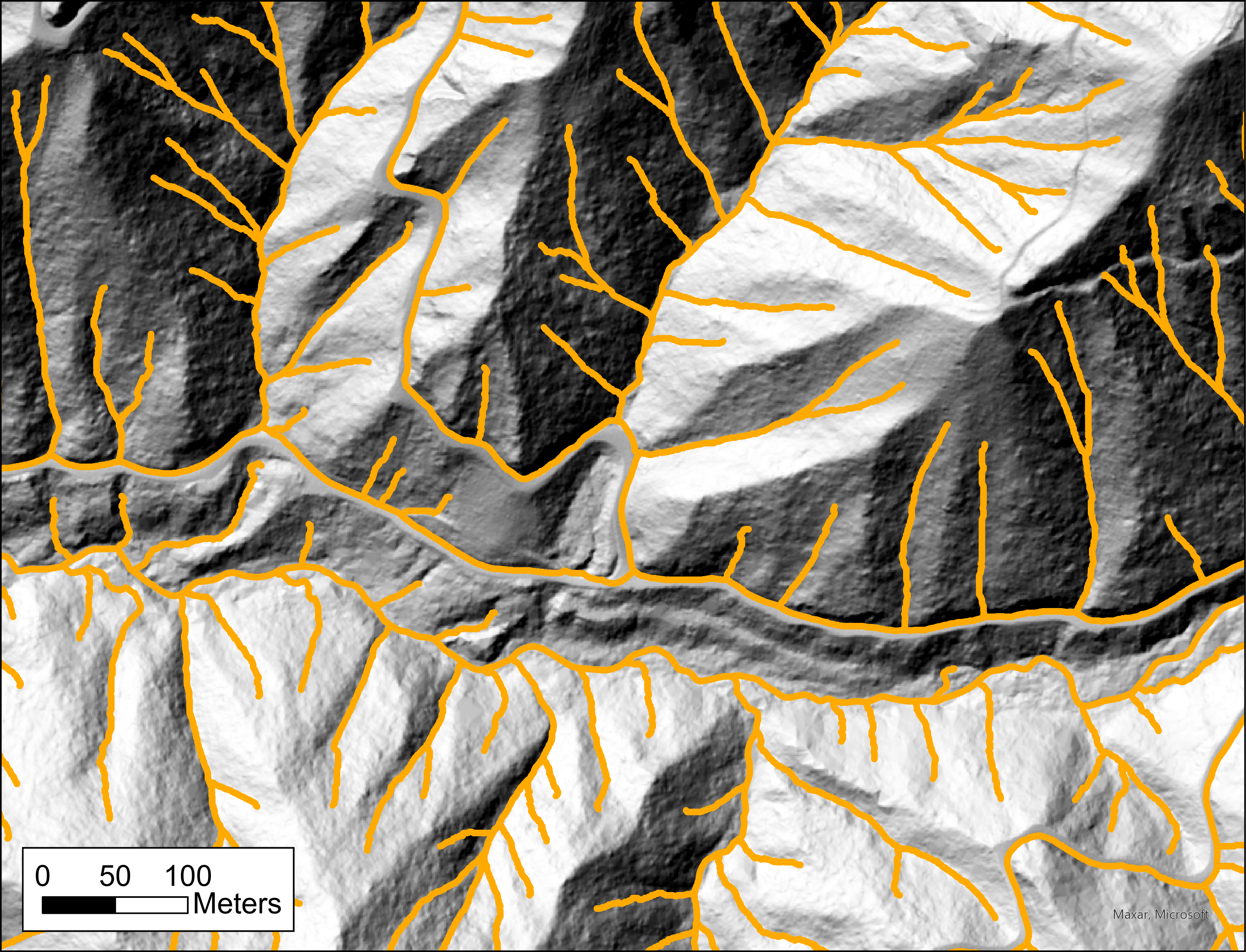
Typically, such other data sources are not available and the likely locations of culverts need to be manually digitized. This task is iterative: building a stream layer, looking for diversions, digitizing a culvert or drainage location, rebuilding the stream layer, and repeating until satisfied with the stream layer. Such manually digitized drainage structures are illustrated for the area shown in Figure 3.7 in Figure 3.8 below.
3.6 Typical Workflow
With high-resolution DEMs, a default strategy for channel initiation and flow-path routing is:
Run program bldgrds with the “CALIBRATE” keyword (see Chapter 1). This will generate a .csv file with the channel density as a function of the ASe threshold value. Use this to determine appropriate threshold values (one for steep terrain, another for low-gradient terrain) for the DEM. The default exponent is 2 (as suggested in Montgomery and Foufoula-Georgiou 1993), but this can be changed to any desired value. A calibration run of bldgrds will also create a binary floating point raster (threshold_ID.flt) showing the ASe value for each DEM cell.
Use program makegrids to create hillslope-gradient and tangential-curvature rasters for the DEM. Use program DEV to produce a Deviation from Mean Elevation (DEV) raster. Use length scales that span several DEM cells and wider than the smallest channels you want to resolve. For a 1-m DEM, 10 to 15 meter length scales work well. Plot these rasters, along with the threshold raster created by bldgrds, over a shaded relief image. Experiement with different threshold values to get a sense of how the upslope extent of mapped channels will vary with the chosen thresholds. Also evaluate these overlays to determine an appropriate minimum flow length overwhich the thresholds need to be met for channel initiation. Channel initiation.
If there are large rivers and water bodies in the study area, you may want to build a water mask for these areas. This can be done using program waterMaskByTopo, which uses the infrared band of NAIP imagery to identify open water. The water mask can be used with bldgrds to guide channel flow paths through these areas. There may be other sources of data for a water mask, such as the 2-D breaklines used to build river and lake polygons for the USGS 3DEP program.
Run program bldgrds with the threshold values for ASe, DEV, and tangential curvature determined in step 2 above. Bldgrds will generate raster files for flow direction and accumulation and a point shapefile of the channel nodes that compose the channel network. Evaluate the channel extent and resulting channel density, and adjust threshold values if needed. Use the node shapefile and the flow accumulation raster to identify flow diversions at roads and manually digitize a road-crossing polyline shapefile. Identify errors in channel courses and manually digitize corrections to use as a channel mask.
Run bldgrds again with the adjusted thresholds, and the water mask, channel mask, and road-crossing shapefiles. Check the output channel network. Repeat until no further issues are identified.
Bldgrds stores the output channel network in a binary data file called nodeNet_ID.dat. This is now available for all other NetStream programs.