Prerequisites

Data structures

When considering how to use these programs, it is helpful to understand how they store and use information. With that understanding, you will have an idea of how to phrase the questions you ask of the models implemented in these programs. The underlying conceptual model is that of a virtual watershed (Barquin et al. 2015). A virtual watershed is a digital data structure that characterizes physical attributes (e.g., topography, land cover) over all points and establishes the pathways and processes by which those points are connected. A Digital Elevation Model (DEM) provides the spatial template and sets the spatial grain (the finest scale at which any attribute is resolved). A channel network traced from the DEM provides the spatial reference: all locations (DEM grid points or cells) are referenced in terms of their relationship to the channel network.

The channel network is recorded digitally using a linked-node-list data structure. Channel courses traced from the DEM extend step-by-step from one DEM grid point to an adjacent point. Each DEM grid point defines a node along the channel course. Each node can reference the adjacent upstream and downstream nodes. Hence, flow paths can be followed both up- and down-stream throughout the DEM.

Channel nodes

Each channel node has an associated list of attributes with information about the point along the channel represented by that node. These attributes include basic information about the channel itself, such as elevation, gradient, and contributing area. They may include information about the contributing area, such as annual precipitation, land cover, and geology.

Importantly, each DEM grid point, and its corresponding cell, is associated with one or more channel nodes. The associated node, or nodes, may be determined from the gravity-driven flow path as determined from the topography inferred from the DEM- the path that surface water flowing over the ground surface would follow from the DEM grid point to the channel. Each DEM grid point thus has an associated set of attributes relating it to the channel network, including flow distance to the channel it drains to and attributes of that channel, such as size, gradient, and sediment transport capacity.

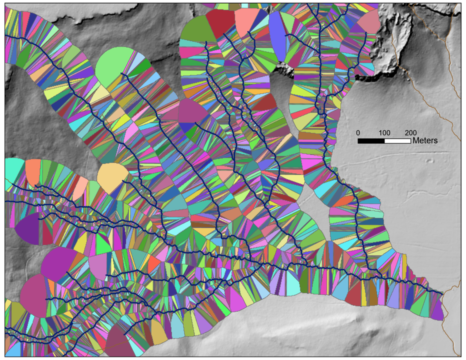
Likewise, each channel node has an associated channel-adjacent contributing area defined by those flow paths. These channel-adjacent areas extend outward from the node to each side of the channel, like wings. They are referred to as drainage wings.

Drainage wings for a portion of a headwater basin in the Sprague River watershed, in southern Oregon.

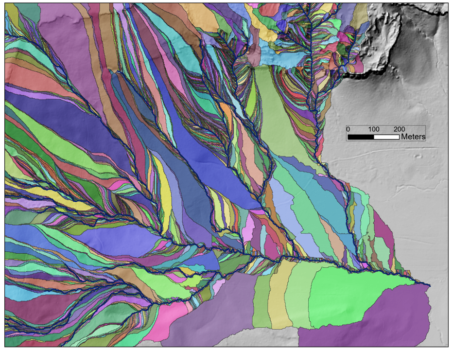
Drainage wings provide a unique discretization of a watershed referenced to the channel network. Attributes of a wing can be assigned to its associated node, including basic measures such as its size and land cover. These attributes may include modeled values, such as estimates of the sediment and organic inputs a wing may provide to the channel. We can divide roads into segments based on intersections with the drainage wings, thus parsing a road network in terms of its potential connectivity with the channel network.

Flow paths provide indicators of hydrologic connectivity, needed for characterizing processes involving movement of water and water-carried material through a watershed. Other types of processes may require other measures of connectivity, such as the Euclidean (straight line) distance from a DEM grid point to a channel.

Parsing of DEM cells based on the closest channel node.

Use of a linked list of channel nodes and discretization of a watershed in terms of associated channel nodes provides an efficient data structure for routing of information across a watershed. The DEM-traced channel network is the framework on which this structure is built, reflected in the name NetStream. The first step for almost all NetStream analyses is creation of that channel network, performed by the program bldgrds. Subsequent programs can read the channel node list created by bldgrds to perform a variety of analyses and to write output shapefiles and raster files readable by a GIS. These programs are listed and described starting with 1  Bldgrds.

Input Files

Programs in the NetStream suite all use ASCII (text) input files with a similar file structure and format. The input files specify any input and output file names and locations, specify the tasks to be performed, and provide any parameter values needed to perform those tasks.

Keywords and arguments

Input files use a “keyword: argument(s)” format. The keyword indicates either what the following arguments are for or indicates a specific task or program option. Entries are identified as a keyword by the following colon (:); any needed arguments follow the keyword; multiple arguments are separated by commas; and if an argument specifies a numerical or logical parameter name, its value is specified after an equal sign. A pound sign (#) indicates a comment; any unrecognized entries are ignored (so if you misspell a keyword, it will be ignored).

Here is an example keyword: argument pair:

DEM: c:\data\Snoqualmie\elev_snoqualmie

This is an input line used by many of the programs. It specifies the DEM file to use. The keyword “DEM” is indicated by the colon; the following argument specifies the location (c:\data\Snoqualmie\) and name (elev_snoqualmie) of the DEM file.

Several things to note about DEM files

1. NetStream programs use a default file name “elev_ID” for DEMs. The “ID” indicates the dataset name. The programs strip off the ID when the “elev_ID” format is used. Subsequent output files that use default names then get the same ID suffix.
2. The full path is required when specifying a DEM file. The programs strip off the path when reading this input line. Any other DEM-related files required by the program are then looked for in the folder specified by the path.
3. NetStream programs can only read three raster-file formats:
   • binary floating point (.flt)
   • tiff, but only uncompressed or those with LZW compression
   • BIL single band (.bil)
4. If no extension is included, the file is assumed to be .flt. If an .flt file with that name cannot be found, the program will look for a file with .tif extension.

Here’s an example with multiple arguments:

OUTPUT NODE POINT SHAPEFILE: c:\data\Snoqualmie\node_test, SPLITS = 4

Here the keyword, or in this case, the keyword phrase (OUTPUT NODE POINT SHAPEFILE) specifies an output file to create. The first argument (c:\data\Snoqualmie\node_test) specifies the location and name of the shapefile to create. The second argument (SPLITS = 4) specifies that the output should be split into four separate shapefiles (this is needed because, for large datasets, ArcGIS can only read shapefile attribute tables of two Gbytes or less).

Important

Keywords and arguments are case sensitive.

Each program has a specific set of keyword: argument pairs that it recognizes. I’ll describe these in the chapters describing the programs.

Attribute lists

For programs that generate output GIS vector files, either point or polyline shapefiles, the data fields to include in the attribute table are specified with an attribute list. An attribute list is initialized with the “ATTRIBUTE LIST” keyword; the “END LIST” keyword flags the end of the list. Here’s an example:

#===================================
ATTRIBUTE LIST:
#———————————————————–
ID:
LENGTH:
CONTRIBUTING AREA: OUTPUT FIELD = AREA_SQKM
MEAN ANNUAL PRECIP: FILE = c:/work/data/wrangell/precip_utm8n, OUTPUT FIELD = MNANPRC_M
VALLEY WIDTH: CHANNEL DEPTHS = 5.0, OUTPUT FIELD = VAL5CW
#———————————————————–
END LIST:
#===================================

Each keyword within the list specifies an output data field. These are generally attributes recognized by the program and will trigger a call to specific subroutines for calculating the attribute values. If the keyword is not recognized by the program, the data field will be created, but filled with nodata values. A full description of the data-field options available is provided in 2  Attribute Lists.

Equations

A data field specified in an attribute list may be defined by an equation using other data fields in the attribute list. Equations are of the form:

\[ y = \beta_0 + \beta_1x_{1.1}^{e_{1.1}}x_{1.2}^{e_{1.2}}... + \beta_2x_{2.1}^{e_{2.1}}x_{2.2}^{e_{2.2}}... \]

Here, the \(\beta_i\) and \(e_{i.j}\) are empirical coefficients and the \(x_{i.j}\) are data-field variables included elsewhere the attribute list. A data-field entry is flagged as an equation by the “EQUATION” argument. The next line(s) specify the constant term \(\beta_0\) with the CONSTANT keyword and each \(\beta_ix_{i.j}^{e_{i.j}}\) term with the TERM keyword. The equation entries are terminated by the END EQUATION keyword. Here is an example:

#==================================
ATTRIBUTE LIST:
#———————————————————-
CONTRIBUTIND AREA: OUTPUT FIELD = AreaSQKM
MEAN ANNUAL PRECIP: FILE = c:\prism\prism_utm10n, OUTPUT FIELD = MnAnPrcM # mean annual precipitation in meters depth
MEAN ANNUAL FLOW: OUTPUT FIELD = MeanAnnCMS, EQUATION # mean annual flow in cubic meters per second
TERM: FIELD = AREA_SQKM, COEF = 0.014, EXPONENT = 0.99, FIELD = MNANPRC_M, EXPONENT = 1.59
END EQUATION:
#——————————————————–
END LIST:
#===================================

In this case, the attribute for mean annual flow (MeanAnnCMS) is defined by the equation

\[ MeanAnnCMS = 0.01454(AreaSQKM^{0.99})(MnAnPrcM^{1.593}) \]

where AreaSQKM is contributing area and MnAnPrcM is mean annual precipitation. If there were a constant term \((\beta_0)\), it would be specified by a line with keyword “CONSTANT:” followed by an argument with the value. If there were additional \(\beta_ix_{i.j}^{e_{i.j}}\) terms, these would be specified by additional lines with a “TERM:” keyword. This format allows specification of a large variety of equation forms.

Raster lists

Data-field attributes can also be calculated from analysis of raster files. For example, we can define a data field that gives the mean gradient or the proportion of the contributing area within each land-cover class over the contributing area to each node, if a gradient or land-cover raster are provided. These tasks are specified using a raster list, initiated with the “RASTER LIST:” keyword.

File Formats

NetStream programs can read binary floating point (.flt) raster files. Uncompressed tiff (.tif) files, and tiff files with LZW compression, can also be read. Certain programs can read binary interleaved by line (.bil) raster files. Raster file names can be specified in the ascii input file without the extension. The programs will look first for an “.flt” file. If none is found, it will look for a “.tif” file.

NetStream programs can read point, polyline, polylineZ, and polygon shapefiles. No extension is needed in the file name.

NetStream programs can currently only write floating point binary (.flt) raster files and point, polyline, and polylineZ shapefiles.

When other file formats are required, these files must be converted, which any GIS can do, or using GDAL (which can be called within python and R).

Barquin, José, Lee E. Benda, Ferdinando Villan, Lee E. Brown, Nuria Bonada, David R. Vietes, Tom J. Battin, et al. 2015. “Coupling Virtual Watersheds with Ecosystem Services Assessment: A 21st Century Platform to Support River Research and Management.” WIREs Water 2 (6): 609–21. https://doi.org/10.1002/wat2.1106.